remotes::install_github("mark-andrews/immr-rpkg")Random Effects Models
Abstract
Multilevel models are, in a fundamental sense, models of models. This guide introduces the idea through the binomial random effects model, building from a single-group binomial through pooled and unpooled estimates to a full multilevel model that treats the per-group log-odds as draws from a common normal distribution. The immr package is used throughout to keep the machinery transparent. Key concepts covered are partial pooling, shrinkage, the prediction interval for a new group, and the role of the between-group standard deviation tau.
Installation
The immr package provides a single function, binomial_model(), that handles all four model types covered in this guide. Install it from GitHub before proceeding.
library(tidyverse)
library(immr)
The rats tumour data
We will work with a classic dataset from Gelman et al. consisting of 71 batches of rats. For each batch we have the number of rats \(n_j\) and the number that developed endometrial stromal polyps \(m_j\).
rats_df <- rats
rats_df
# A tibble: 71 × 3
batch m n
<dbl> <dbl> <dbl>
1 1 0 20
2 2 0 20
3 3 0 20
4 4 0 20
5 5 0 20
6 6 0 20
7 7 0 20
8 8 0 19
9 9 0 19
10 10 0 19
# ℹ 61 more rowsEach row is one batch. The sample proportion \(m_j/n_j\) varies substantially across batches, partly because the true tumour probabilities differ and partly because the batch sizes are small, which amplifies sampling noise.
A single-group model
Begin by focusing on batch 42 alone.
rats_42 <- filter(rats_df, batch == 42)
rats_42
# A tibble: 1 × 3
batch m n
<dbl> <dbl> <dbl>
1 42 2 13The natural model is binomial: the number of tumours \(m\) in a batch of size \(n\) is a draw from \(\mathrm{Binom}(\theta, n)\), where \(\theta\) is the unknown probability of a tumour.
M1 <- binomial_model(m, n, data = rats_42)
M1
Binomial model (pooled)
Estimate : 0.1538
95% CI : [0.0387, 0.4506]The estimate and its 95% confidence interval are returned on the probability scale directly.
A pooled model
Now apply the same model to all 71 batches simultaneously, treating them as one large batch with a single shared probability.
M2 <- binomial_model(m, n, data = rats_df)
M2
Binomial model (pooled)
Estimate : 0.1535
95% CI : [0.1373, 0.1713]This assumes that every batch has exactly the same tumour probability. The estimate is the pooled proportion across all rats. It ignores the fact that batches are distinct biological units with their own rates.
An unpooled model
The opposite extreme is to estimate a separate probability for each batch, treating the batches as entirely independent.
M3 <- binomial_model(m, n, group = batch, data = rats_df)
M3$estimates
# A tibble: 71 × 4
group estimate lower upper
<chr> <dbl> <dbl> <dbl>
1 1 0 0 0.161
2 2 0 0 0.161
3 3 0 0 0.161
4 4 0 0 0.161
5 5 0 0 0.161
6 6 0 0 0.161
7 7 0 0 0.161
8 8 0 0 0.168
9 9 0 0 0.168
10 10 0 0 0.168
# ℹ 61 more rowsEach row gives the maximum likelihood estimate and confidence interval for one batch. Several batches have \(m_j = 0\), which would push the log-odds MLE to \(-\infty\) and produce degenerate Wald intervals. binomial_model() uses Wilson score intervals in the unpooled case, which remain well-behaved at the boundaries.
A multilevel model
The pooled model ignores between-batch variation entirely; the unpooled model ignores the fact that the batches are all part of the same experiment. The multilevel model takes a middle position. It assumes that the log-odds parameters \(\beta_1, \beta_2, \ldots, \beta_J\) for the 71 batches are not independent but are drawn from a common normal distribution:
\[ \beta_j \sim N(b, \tau^2). \]
This can equivalently be written \(\beta_j = b + \xi_j\) where \(\xi_j \sim N(0, \tau^2)\), so the model for each batch becomes
\[ m_j \sim \mathrm{Binom}(\theta_j, n_j), \qquad \log\!\left(\frac{\theta_j}{1-\theta_j}\right) = b + \xi_j. \]
The normal distribution \(N(b, \tau^2)\) is a model of the population from which the batch-specific log-odds are drawn. This is what makes it a multilevel model: the individual batch models are themselves modelled.
M4 <- binomial_model(m, n, group = batch, data = rats_df, multilevel = TRUE)
M4
Binomial model (multilevel)
Grand mean : 0.1260 [0.1021, 0.1545] (95% CI)
Prediction int : [0.0377, 0.3465] (95% PI for new group)
Mu : -1.9369 (grand mean, log-odds)
Tau : 0.6646 (random-effects SD, log-odds)
Group estimates (partial pooling):
# A tibble: 71 × 4
group estimate lower upper
<chr> <dbl> <dbl> <dbl>
1 1 0.0713 0.0259 0.182
2 2 0.0713 0.0259 0.182
3 3 0.0713 0.0259 0.182
4 4 0.0713 0.0259 0.182
5 5 0.0713 0.0259 0.182
6 6 0.0713 0.0259 0.182
7 7 0.0713 0.0259 0.182
8 8 0.0727 0.0262 0.186
9 9 0.0727 0.0262 0.186
10 10 0.0727 0.0262 0.186
# ℹ 61 more rowsThe output gives:
- The grand mean \(b\) on the probability scale, with a confidence interval.
- The prediction interval for a new batch drawn from the same population.
- \(\tau\) — the standard deviation of the batch-specific log-odds.
- Per-batch estimates based on partial pooling.
Partial pooling and shrinkage
The multilevel model neither ignores between-batch structure (pooled) nor treats each batch in isolation (unpooled). It performs partial pooling: the estimate for each batch is a weighted average of its own data and the grand mean, with the weights determined by the relative precision of the two sources of information.
The consequence is shrinkage: the multilevel estimates are pulled towards the grand mean compared to the unpooled estimates. Batches with small \(n_j\) or extreme proportions experience the most shrinkage.
unpooled <- M3$estimates |>
  rename(unpooled = estimate)

multilevel <- M4$estimates |>
  rename(multilevel = estimate)

comparison <- left_join(unpooled, multilevel, by = "group") |>
  select(group, unpooled, multilevel)

comparison |>
  pivot_longer(-group, names_to = 'type', values_to = 'estimate') |>
  ggplot(aes(x = type, y = estimate, group = group)) +
  geom_point() +
  geom_line() +
  labs(x = 'Model type', y = 'Estimate')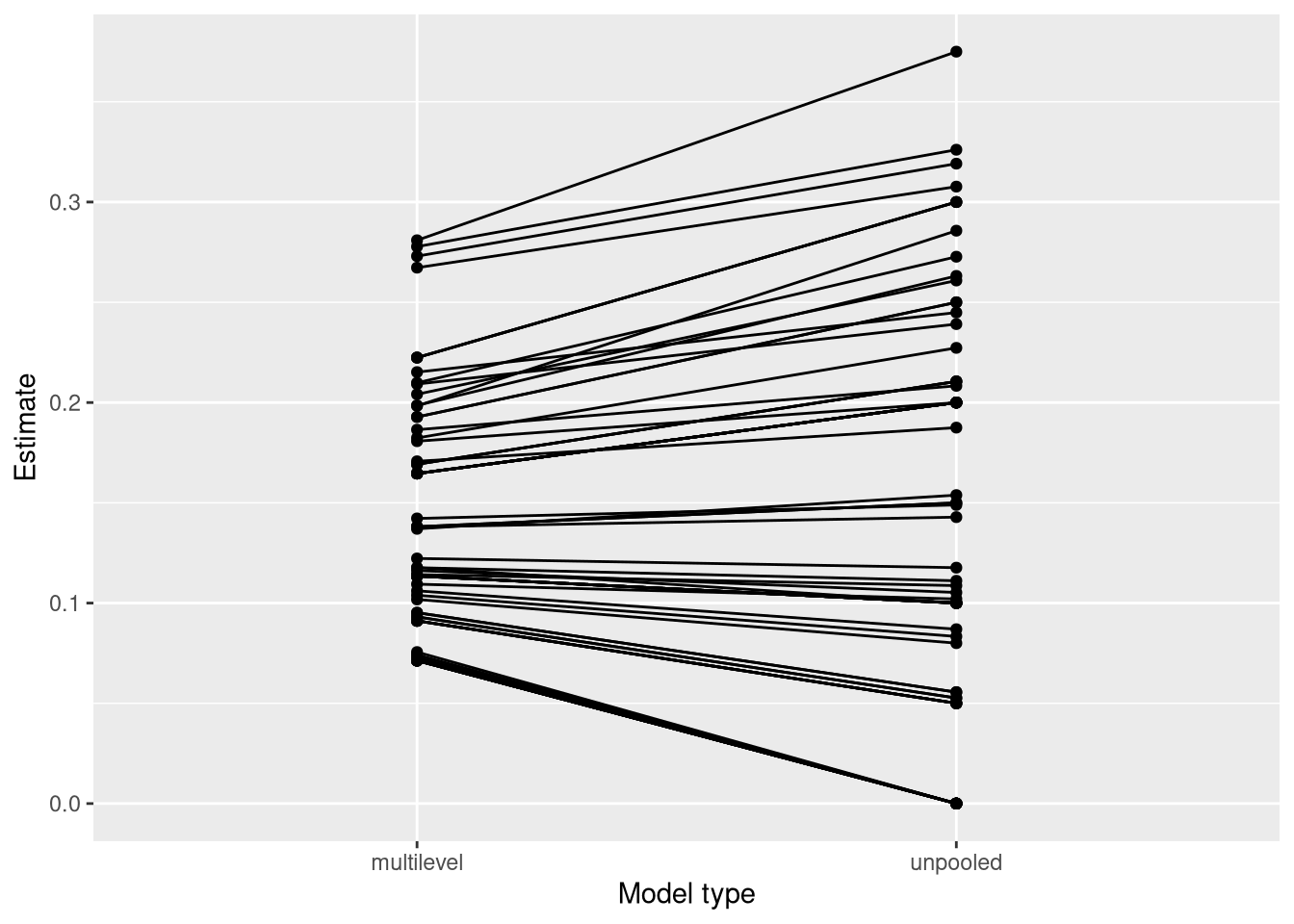
Points above the diagonal line are batches whose multilevel estimate is higher than the unpooled estimate; points below it are batches whose multilevel estimate is lower. Both cases represent the multilevel estimate being pulled towards the grand mean.
The population distribution
The multilevel model provides a distribution over the probability parameter for the entire population of batches, including future ones not yet observed. This is recovered from the grand mean and \(\tau\).
b <- M4$mu
tau <- M4$tau

theta_seq <- seq(0.001, 0.999, length.out = 1000)
log_odds <- log(theta_seq / (1 - theta_seq))
jacobian <- abs(1 / theta_seq + 1 / (1 - theta_seq))
density <- dnorm(log_odds, mean = b, sd = tau) * jacobian

tibble(theta = theta_seq, density = density) |>
  ggplot(aes(x = theta, y = density)) +
  geom_line() +
  labs(
    x = expression(theta),
    y = "Density",
    title = "Estimated population distribution of tumour probabilities"
  )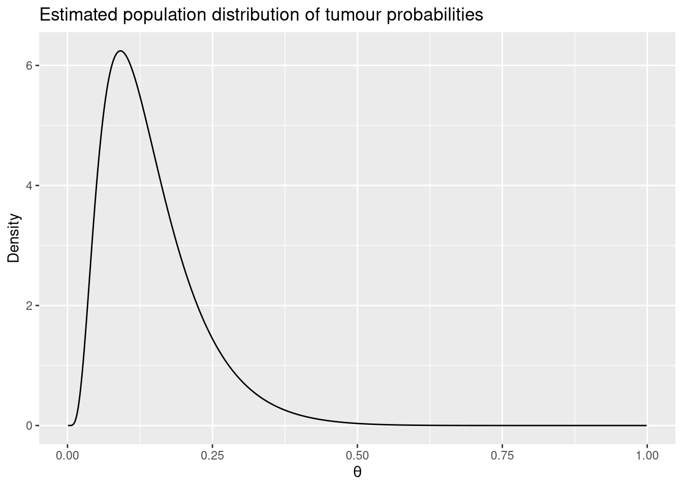
The prediction interval in M4$prediction_int gives the range within which a new batch’s probability is expected to fall with 95% probability, according to this population model.
Why the multilevel model is preferable
The unpooled model treats each batch as a separate problem, discarding the information that batches come from the same experiment. For batches with very few rats, this produces wide and sometimes degenerate confidence intervals. The multilevel model borrows strength across batches: even a batch with a single rat gets a reasonable estimate, because the population-level distribution regularises the inference.
At the same time, the multilevel model does not ignore real between-batch variation. If \(\tau\) is large, the estimates remain spread out. If \(\tau\) is near zero, the model converges to the fully pooled result. The estimate of \(\tau\) from the data automatically determines how much pooling is appropriate.