library(tidyverse)
library(lme4)
library(immr)Normal Random Effects Models
Abstract
When grouped data are continuous rather than binary, the natural multilevel model is the normal random effects model. This guide works through per-capita alcohol consumption data across countries, building from a single-country normal model through a non-multilevel fixed-effects model to a full multilevel model fitted with lmer. The intraclass correlation coefficient is derived from the estimated variance components, and the shrinkage behaviour is illustrated by comparing multilevel and non-multilevel country estimates.
The alcohol data
The dataset records per-capita annual alcohol consumption (litres of pure alcohol) in 190 countries across multiple years.
alcohol_df <- alcohol
alcohol_df
# A tibble: 411 × 3
country year alcohol
<fct> <dbl> <dbl>
1 Russia 1985 13.3
2 Russia 1986 10.8
3 Russia 1987 11.0
4 Russia 1988 11.6
5 Russia 1989 12.0
6 Chile 1990 9.43
7 Ecuador 1990 8.4
8 Greece 1990 12.5
9 Russia 1990 12.3
10 Russia 1991 12.7
# ℹ 401 more rowsThe data has a grouped structure: multiple observations per country, one per year. We want to model the average consumption for each country, accounting for the fact that year-to-year variation within a country is different from country-to-country variation.
A single-country model
Begin with Russia alone.
russia_df <- filter(alcohol_df, country == "Russia")
russia_df
# A tibble: 12 × 3
country year alcohol
<fct> <dbl> <dbl>
1 Russia 1985 13.3
2 Russia 1986 10.8
3 Russia 1987 11.0
4 Russia 1988 11.6
5 Russia 1989 12.0
6 Russia 1990 12.3
7 Russia 1991 12.7
8 Russia 1992 13.2
9 Russia 1993 13.6
10 Russia 1994 13.3
11 Russia 2005 15.8
12 Russia 2008 16.2The simplest model treats the annual values as draws from a normal distribution with an unknown mean and standard deviation.
M5 <- lm(alcohol ~ 1, data = russia_df)
coef(M5)
(Intercept)
12.9775 sigma(M5)[1] 1.688394The intercept is the estimated mean consumption; sigma is the estimated standard deviation of year-to-year variation within Russia.
The non-multilevel model for all countries
Extending this to all countries at once with no multilevel structure gives one mean per country, each estimated independently.
M_flat <- lm(alcohol ~ 0 + country, data = alcohol_df)This is a one-way ANOVA model. Each country gets its own mean, and all within-country variances are constrained to be equal. The countries are treated as entirely separate problems.
The multilevel model
The multilevel model adds a distributional assumption on the country means. If \(y_i\) is the alcohol consumption for observation \(i\), and \(x_i\) indicates which of the \(J\) countries it belongs to, the model is:
\[ \begin{aligned} y_i &\sim N(\mu_{[x_i]}, \sigma^2), \\ \mu_j &\sim N(\phi, \tau^2), \quad j = 1, \ldots, J. \end{aligned} \]
The country means \(\mu_1, \ldots, \mu_J\) are not treated as fixed unknowns but as draws from a normal distribution with grand mean \(\phi\) and standard deviation \(\tau\). Writing \(\mu_j = \phi + \xi_j\) where \(\xi_j \sim N(0, \tau^2)\) gives the equivalent form
\[ y_i = \phi + \xi_{[x_i]} + \epsilon_i, \quad \epsilon_i \sim N(0, \sigma^2), \]
which makes the two sources of variance explicit: \(\tau^2\) is the between-country variance and \(\sigma^2\) is the within-country (year-to-year) variance.
This is fitted with lmer.
M6 <- lmer(alcohol ~ 1 + (1 | country), data = alcohol_df)
summary(M6)
Linear mixed model fit by REML ['lmerMod']
Formula: alcohol ~ 1 + (1 | country)
Data: alcohol_df
REML criterion at convergence: 1918.2
Scaled residuals:
Min 1Q Median 3Q Max
-3.4661 -0.1582 -0.0719 0.1642 5.9576
Random effects:
Groups Name Variance Std.Dev.
country (Intercept) 22.208 4.713
Residual 1.108 1.053
Number of obs: 411, groups: country, 189
Fixed effects:
Estimate Std. Error t value
(Intercept) 6.6612 0.3469 19.2The Fixed effects section gives \(\hat{\phi}\), the estimated grand mean. The Random effects section gives the estimated \(\tau\) (labelled Std.Dev. under country) and \(\sigma\) (labelled Std.Dev. under Residual).
Extract these directly.
phi   <- fixef(M6)
tau   <- sqrt(as.numeric(VarCorr(M6)$country))
sigma <- sigma(M6)

phi
(Intercept)
6.661225 tau[1] 4.712518sigma[1] 1.052532The country-level means are available from coef and the country-level deviations \(\xi_j\) from ranef.
coef(M6)$country |> head() (Intercept)
Afghanistan 0.1864940
Albania 6.9771209
Algeria 0.9670258
Andorra 12.6750032
Angola 5.5136237
Antigua and Barbuda 7.6698429ranef(M6)$country |> head() (Intercept)
Afghanistan -6.4747314
Albania 0.3158955
Algeria -5.6941995
Andorra 6.0137779
Angola -1.1476016
Antigua and Barbuda 1.0086175The intraclass correlation coefficient
Each observation \(y_i\) has variance \(\tau^2 + \sigma^2\): some variance comes from countries differing from one another and some from year-to-year fluctuation within each country. The proportion of the total variance attributable to between-country differences is the intraclass correlation coefficient (ICC):
\[ \mathrm{ICC} = \frac{\tau^2}{\tau^2 + \sigma^2}. \]
tau^2 / (tau^2 + sigma^2)[1] 0.9524858An ICC close to 1 means that most of the variation is between countries (countries differ a great deal from each other, but each country is consistent across years). An ICC close to 0 means that most of the variation is within countries (year-to-year fluctuation dominates country-to-country differences).
The ICC also tells us about the degree of clustering: observations from the same country are not independent. Two observations from the same country have correlation equal to the ICC.
Shrinkage
As with the binomial random effects model, the multilevel estimates are shrunk towards the grand mean \(\phi\) relative to the non-multilevel (flat) estimates.
flat_estimates <- coef(M_flat) |>
  enframe(name = "country", value = "flat") |>
  mutate(country = str_remove(country, "^country"))

multilevel_estimates <- coef(M6)$country |>
  rownames_to_column("country") |>
  rename(multilevel = `(Intercept)`)

comparison <- inner_join(flat_estimates, multilevel_estimates, by = "country")

ggplot(comparison, aes(x = flat, y = multilevel)) +
  geom_point(alpha = 0.5) +
  geom_abline(slope = 1, intercept = 0, linetype = "dashed") +
  labs(
    x = "Non-multilevel estimate",
    y = "Multilevel estimate",
    title = "Shrinkage of country means toward the grand mean"
  )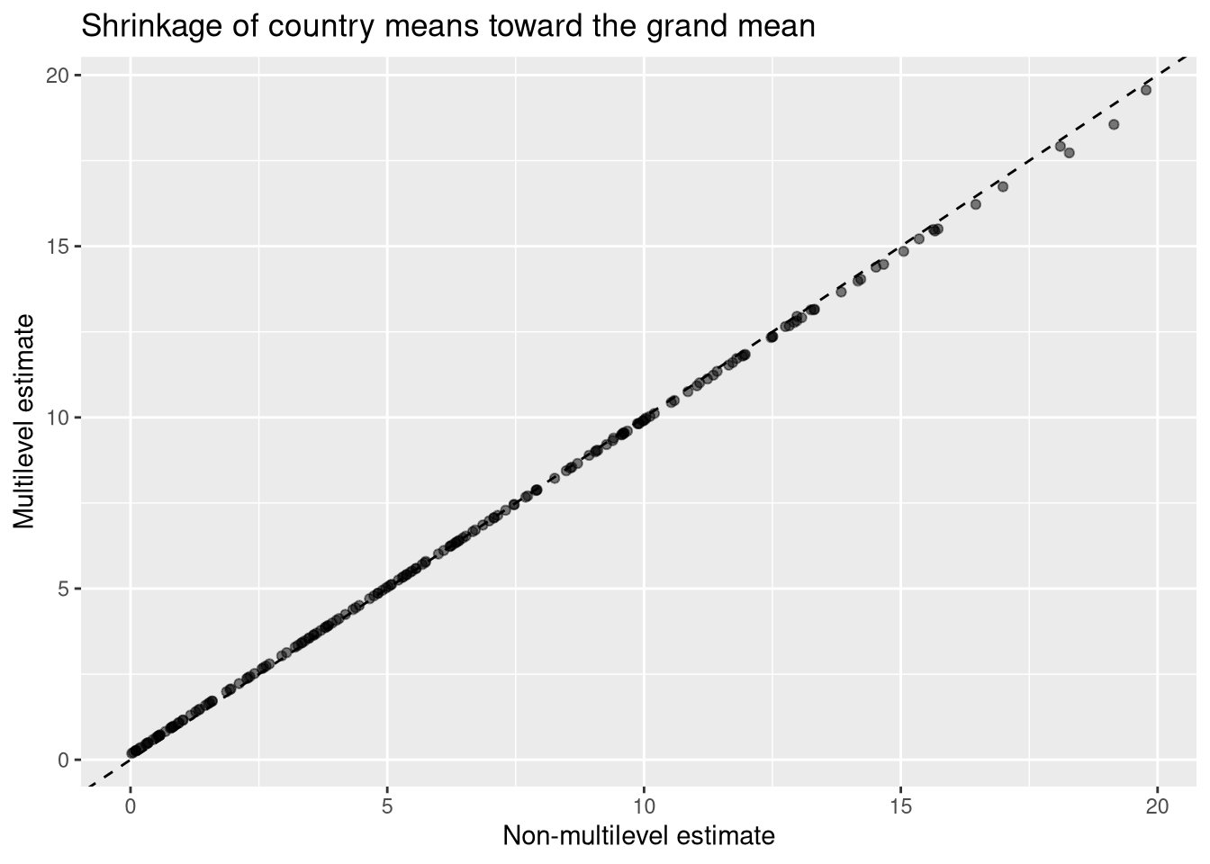
In this dataset \(\tau\) is large relative to \(\sigma\) — countries differ substantially and consistently from one another — so the ICC is relatively high and the shrinkage effect is modest. Each country’s data is informative enough that the grand mean contributes little.
Confidence intervals
The confint function provides confidence intervals for all parameters of the fitted model, including the variance components.
confint(M6)Computing profile confidence intervals ... 2.5 % 97.5 %
.sig01 4.2513053 5.228805
.sigma 0.9616978 1.158629
(Intercept) 5.9795531 7.342833The rows .sig01 and .sigma correspond to \(\tau\) and \(\sigma\) respectively, and (Intercept) to \(\phi\).