library(tidyverse)
library(lme4)
library(modelr)
library(immr)Linear Mixed Effects Models
Abstract
The linear mixed effects model extends the random effects framework to regression, allowing both the intercept and slope of a predictor to vary across groups. This guide develops the model using the pvtrt data from immr, moving from a single-subject regression through a non-multilevel flat model to the full varying-intercepts and varying-slopes multilevel model. It covers the fixed-versus-random effects decomposition, the four main model variants (full, varying intercepts only, varying slopes only, no-correlation), model comparison using likelihood ratio tests, and inference via confidence intervals and lmerTest.
The sleep deprivation data
The pvtrt dataset from immr records the average reaction time (ms) of 18 participants across 10 days of a sleep deprivation experiment. On day 0, participants had normal sleep; from day 1 onward, they were restricted to 3 hours per night.
pvtrt# A tibble: 180 × 3
rt day id
<dbl> <dbl> <fct>
1 250. 0 s1
2 259. 1 s1
3 251. 2 s1
4 321. 3 s1
5 357. 4 s1
6 415. 5 s1
7 382. 6 s1
8 290. 7 s1
9 431. 8 s1
10 466. 9 s1
# ℹ 170 more rowsPlotting reaction time against days for each participant reveals that most slow down over time, but the rate of slowing varies considerably.
ggplot(pvtrt, aes(x = day, y = rt)) +
  geom_point() +
  stat_smooth(method = "lm", se = FALSE) +
  facet_wrap(~id) +
  labs(x = "Day", y = "Reaction time (ms)")
`geom_smooth()` using formula = 'y ~ x'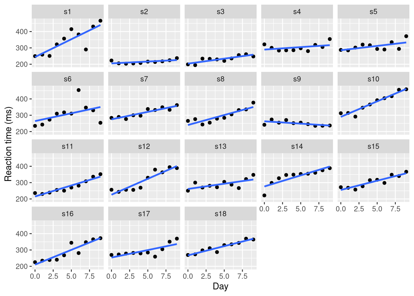
A single-subject model
A simple normal linear model for one subject captures their individual trend.
M_s12 <- lm(rt ~ day, data = filter(pvtrt, id == "s12"))
coef(M_s12)
(Intercept) day
225.83460 19.50402 This participant’s reaction time increases by approximately 19.5 ms per day of sleep deprivation, with a baseline of 225.8 ms.
The non-multilevel flat model
Fitting a separate regression to every subject simultaneously, with no multilevel structure, is the non-multilevel varying-intercepts-and-slopes model.
M_flat <- lm(rt ~ 0 + id + id:day, data = pvtrt)The 0 + id part gives one intercept per participant; id:day gives one slope per participant. This is equivalent to 18 independent linear regressions sharing only the residual variance \(\sigma^2\).
The linear mixed effects model
The multilevel version assumes that the vector of coefficients \(\boldsymbol{\beta}_j = (\beta_{j0}, \beta_{j1})^\top\) for subject \(j\) is drawn from a bivariate normal distribution:
\[ \begin{aligned} y_i &\sim N(\mu_i, \sigma^2), \\ \mu_i &= \beta_{[s_i]0} + \beta_{[s_i]1} x_i, \\ \boldsymbol{\beta}_j &\sim N(\boldsymbol{b}, \Sigma), \quad j = 1, \ldots, J. \end{aligned} \]
Here \(\boldsymbol{b} = (b_0, b_1)^\top\) is the population average intercept and slope, and \(\Sigma\) is the \(2 \times 2\) covariance matrix of subject-to-subject variation. Writing \(\boldsymbol{\beta}_j = \boldsymbol{b} + \boldsymbol{\zeta}_j\) where \(\boldsymbol{\zeta}_j \sim N(\boldsymbol{0}, \Sigma)\) gives the fixed-and-random decomposition:
\[ \mu_i = \underbrace{b_0 + b_1 x_i}_{\text{fixed effects}} + \underbrace{\zeta_{[s_i]0} + \zeta_{[s_i]1} x_i}_{\text{random effects}}. \]
The fixed effects are the population-level intercept and slope. The random effects are the subject-specific deviations from those population values. This is why the model is called a linear mixed effects model: it mixes fixed and random components.
M7 <- lmer(rt ~ day + (day | id), data = pvtrt)
summary(M7)
Linear mixed model fit by REML ['lmerMod']
Formula: rt ~ day + (day | id)
Data: pvtrt
REML criterion at convergence: 1743.6
Scaled residuals:
Min 1Q Median 3Q Max
-3.9536 -0.4634 0.0231 0.4634 5.1793
Random effects:
Groups Name Variance Std.Dev. Corr
id (Intercept) 612.10 24.741
day 35.07 5.922 0.07
Residual 654.94 25.592
Number of obs: 180, groups: id, 18
Fixed effects:
Estimate Std. Error t value
(Intercept) 251.405 6.825 36.838
day 10.467 1.546 6.771
Correlation of Fixed Effects:
(Intr)
day -0.138Fixed effects
The fixed effects give the average intercept and slope across all subjects.
fixef(M7)(Intercept) day
251.40510 10.46729 The population average reaction time at baseline (day 0) is 251.4 ms, and the average increase per day of sleep deprivation is 10.5 ms.
Random effects
The random effects structure gives the variance components.
VarCorr(M7) Groups Name Std.Dev. Corr
id (Intercept) 24.7407
day 5.9221 0.066
Residual 25.5918 The standard deviations \(\tau_0\) and \(\tau_1\) describe how much individual subjects vary around the population averages in their intercept and slope respectively. The correlation \(\rho\) describes the tendency for subjects with higher baseline reaction times to also have steeper or shallower slopes.
Participant-specific coefficients
The estimated \(\boldsymbol{\beta}_j\) for each subject can be recovered with coef, which adds the fixed effects to the random effects.
coef(M7)$id |> head() (Intercept) day
s1 253.6637 19.666262
s2 211.0064 1.847605
s3 212.4447 5.018429
s4 275.0957 5.652936
s5 273.6654 7.397374
s6 260.4447 10.195109Compare these to the non-multilevel estimates. The multilevel estimates are shrunk towards the population mean \(\boldsymbol{b}\): subjects with extreme slope or intercept values in the flat model are pulled back towards the population centre.
Visualisation
add_predictions(pvtrt, M7) |>
  ggplot(aes(x = day, y = rt, colour = id)) +
  geom_point() +
  geom_line(aes(y = pred)) +
  facet_wrap(~id) +
  theme(legend.position = "none") +
  labs(y = "Reaction time (ms)")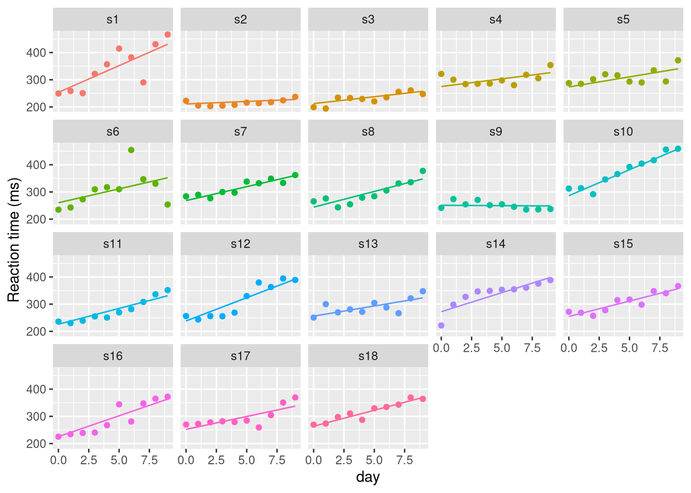
Model variants
Varying intercepts only
This model allows only the intercept to vary across subjects; the slope is fixed at the population value \(b_1\).
M8 <- lmer(rt ~ day + (1 | id), data = pvtrt)The formula (1 | id) specifies a random intercept per participant with no random slope.
fixef(M8)(Intercept) day
251.40510 10.46729 VarCorr(M8) Groups Name Std.Dev.
id (Intercept) 37.124
Residual 30.991 All subjects share the same slope; only their baselines differ.
Varying slopes only
This model allows only the slope to vary; the intercept is fixed at \(b_0\).
M9 <- lmer(rt ~ day + (0 + day | id), data = pvtrt)The 0 + day syntax suppresses the random intercept.
fixef(M9)(Intercept) day
251.40510 10.46729 VarCorr(M9) Groups Name Std.Dev.
id day 7.260
Residual 29.018 Varying intercepts and slopes, no correlation
The full model (day | id) assumes that random intercepts and slopes can be correlated. To allow both to vary but force them to be independent, use either of these equivalent specifications.
M10a <- lmer(rt ~ day + (1 | id) + (0 + day | id), data = pvtrt)
M10b <- lmer(rt ~ day + (day || id), data = pvtrt)
The || notation is shorthand for specifying independent random effects for all terms.
VarCorr(M10a) Groups Name Std.Dev.
id (Intercept) 25.0513
id.1 day 5.9882
Residual 25.5653 The estimated \(\tau_0\) and \(\tau_1\) are present but \(\rho\) is absent.
Model comparison
To compare models using a likelihood ratio test, both models must be fitted with maximum likelihood rather than REML. REML estimates are preferred for the variance parameters but cannot be used to compare models with different fixed effects structures; they can be used to compare models with the same fixed effects but different random effects structures.
To compare the full model against the no-correlation model, both have the same fixed effects, so REML-based comparison is valid.
anova(M10a, M7)refitting model(s) with ML (instead of REML)Data: pvtrt
Models:
M10a: rt ~ day + (1 | id) + (0 + day | id)
M7: rt ~ day + (day | id)
npar AIC BIC logLik -2*log(L) Chisq Df Pr(>Chisq)
M10a 5 1762.0 1778.0 -876.00 1752.0
M7 6 1763.9 1783.1 -875.97 1751.9 0.0639 1 0.8004The likelihood ratio test assesses whether including the correlation between random intercepts and slopes significantly improves the fit.
To compare the full model against the varying-intercepts-only model, use ML.
M7_ml  <- lmer(rt ~ day + (day | id), data = pvtrt, REML = FALSE)
M8_ml  <- lmer(rt ~ day + (1 | id),   data = pvtrt, REML = FALSE)
M10_ml <- lmer(rt ~ day + (day || id), data = pvtrt, REML = FALSE)

anova(M8_ml, M10_ml, M7_ml)
Data: pvtrt
Models:
M8_ml: rt ~ day + (1 | id)
M10_ml: rt ~ day + ((1 | id) + (0 + day | id))
M7_ml: rt ~ day + (day | id)
npar AIC BIC logLik -2*log(L) Chisq Df Pr(>Chisq)
M8_ml 4 1802.1 1814.8 -897.04 1794.1
M10_ml 5 1762.0 1778.0 -876.00 1752.0 42.0754 1 8.782e-11 ***
M7_ml 6 1763.9 1783.1 -875.97 1751.9 0.0639 1 0.8004
---
Signif. codes: 0 '***' 0.001 '**' 0.01 '*' 0.05 '.' 0.1 ' ' 1Inference
Confidence intervals
Profile-likelihood confidence intervals for the fixed effects and variance parameters are obtained as follows.
confint(M7)Computing profile confidence intervals ... 2.5 % 97.5 %
.sig01 14.3813850 37.7158318
.sig02 3.8011641 8.7533831
.sig03 -0.4815008 0.6849863
.sigma 22.8982669 28.8579965
(Intercept) 237.6806955 265.1295147
day 7.3586533 13.5759188The rows .sig01, .sig02, .sig03 correspond to elements of the Cholesky factor of \(\Sigma\) and .sigma to \(\sigma\). The rows for (Intercept) and day are the fixed effects.
P-values with lmerTest
lme4 deliberately does not provide p-values for fixed effects, because the degrees of freedom for the \(t\)-statistic in a mixed model are not well-defined. The lmerTest package implements the Satterthwaite approximation to the denominator degrees of freedom, which is a widely-used practical solution.
M7_test <- lmerTest::lmer(rt ~ day + (day | id), data = pvtrt)
summary(M7_test)
Linear mixed model fit by REML. t-tests use Satterthwaite's method [
lmerModLmerTest]
Formula: rt ~ day + (day | id)
Data: pvtrt
REML criterion at convergence: 1743.6
Scaled residuals:
Min 1Q Median 3Q Max
-3.9536 -0.4634 0.0231 0.4634 5.1793
Random effects:
Groups Name Variance Std.Dev. Corr
id (Intercept) 612.10 24.741
day 35.07 5.922 0.07
Residual 654.94 25.592
Number of obs: 180, groups: id, 18
Fixed effects:
Estimate Std. Error df t value Pr(>|t|)
(Intercept) 251.405 6.825 17.000 36.838 < 2e-16 ***
day 10.467 1.546 17.000 6.771 3.26e-06 ***
---
Signif. codes: 0 '***' 0.001 '**' 0.01 '*' 0.05 '.' 0.1 ' ' 1
Correlation of Fixed Effects:
(Intr)
day -0.138The p-values appear in the Fixed effects table. Confidence intervals from confint(M7) are the preferred summary for the fixed effects.