library(tidyverse)
library(lme4)
library(modelr)
library(performance)
library(immr)Explained Variance in Multilevel Models
Abstract
The coefficient of determination \(R^2\) is a natural measure of model fit in ordinary linear regression, but it does not extend directly to mixed effects models because predictions can be formed at the population level (from fixed effects only) or at the subject level (from fixed plus random effects combined). This guide derives four equivalent definitions of \(R^2\) in the linear model, shows why the naive extension fails for mixed models, and develops the marginal and conditional \(R^2\) statistics of Nakagawa and Schielzeth, implemented via the performance package.
R² in ordinary linear regression
The coefficient of determination measures the proportion of variance in the outcome that is accounted for by the predictors. For a linear model, four equivalent definitions all produce the same value.
m <- lm(dist ~ speed, data = cars)
summary(m)$r.squared
[1] 0.6510794Definition 1. One minus the ratio of residual variance to outcome variance.
1 - var(residuals(m)) / var(cars$dist)[1] 0.6510794Definition 2. The ratio of explained variance (variance of fitted values) to outcome variance.
var(predict(m)) / var(cars$dist)[1] 0.6510794Definition 3. The ratio of explained variance to total variance, where total variance is the sum of explained and residual variance.
var(predict(m)) / (var(predict(m)) + var(residuals(m)))[1] 0.6510794Definition 4. One minus the ratio of residual variance in the full model to the residual variance in the intercept-only model.
m0 <- lm(dist ~ 1, data = cars)
1 - var(residuals(m)) / var(residuals(m0))
[1] 0.6510794All four are equal.
The complication in mixed effects models
In a mixed effects model, predictions can be formed in two ways.
The marginal prediction uses only the fixed effects: it gives the expected outcome for a hypothetical new individual drawn from the population, without knowing which random effects that individual would have.
The conditional prediction uses both fixed effects and random effects: it gives the expected outcome for a specific individual whose random effects have been estimated.
M7 <- lmer(rt ~ day + (day | id), data = pvtrt)predict(M7) # conditional: fixed + random effects 1 2 3 4 5 6 7 8
253.6637 273.3299 292.9962 312.6624 332.3287 351.9950 371.6612 391.3275
9 10 11 12 13 14 15 16
410.9937 430.6600 211.0064 212.8540 214.7016 216.5492 218.3968 220.2444
17 18 19 20 21 22 23 24
222.0920 223.9396 225.7872 227.6348 212.4447 217.4631 222.4816 227.5000
25 26 27 28 29 30 31 32
232.5184 237.5368 242.5553 247.5737 252.5921 257.6106 275.0957 280.7487
33 34 35 36 37 38 39 40
286.4016 292.0545 297.7075 303.3604 309.0133 314.6663 320.3192 325.9721
41 42 43 44 45 46 47 48
273.6654 281.0628 288.4602 295.8575 303.2549 310.6523 318.0497 325.4470
49 50 51 52 53 54 55 56
332.8444 340.2418 260.4447 270.6398 280.8349 291.0300 301.2251 311.4202
57 58 59 60 61 62 63 64
321.6153 331.8104 342.0055 352.2007 268.2456 278.4893 288.7329 298.9766
65 66 67 68 69 70 71 72
309.2202 319.4639 329.7075 339.9512 350.1948 360.4385 244.1725 255.7144
73 74 75 76 77 78 79 80
267.2562 278.7981 290.3400 301.8818 313.4237 324.9656 336.5074 348.0493
81 82 83 84 85 86 87 88
251.0714 250.7866 250.5017 250.2168 249.9319 249.6470 249.3622 249.0773
89 90 91 92 93 94 95 96
248.7924 248.5075 286.2956 305.3911 324.4867 343.5822 362.6778 381.7733
97 98 99 100 101 102 103 104
400.8689 419.9644 439.0600 458.1556 226.1949 237.8356 249.4763 261.1170
105 106 107 108 109 110 111 112
272.7577 284.3985 296.0392 307.6799 319.3206 330.9613 238.3351 255.4166
113 114 115 116 117 118 119 120
272.4981 289.5796 306.6611 323.7426 340.8241 357.9056 374.9871 392.0686
121 122 123 124 125 126 127 128
255.9830 263.4350 270.8870 278.3390 285.7911 293.2431 300.6951 308.1471
129 130 131 132 133 134 135 136
315.5992 323.0512 272.2688 286.2721 300.2754 314.2786 328.2819 342.2852
137 138 139 140 141 142 143 144
356.2885 370.2918 384.2951 398.2984 254.6806 266.0201 277.3596 288.6991
145 146 147 148 149 150 151 152
300.0386 311.3781 322.7176 334.0571 345.3966 356.7361 225.7921 241.0819
153 154 155 156 157 158 159 160
256.3716 271.6614 286.9512 302.2410 317.5307 332.8205 348.1103 363.4000
161 162 163 164 165 166 167 168
252.2122 261.6913 271.1704 280.6495 290.1287 299.6078 309.0869 318.5661
169 170 171 172 173 174 175 176
328.0452 337.5243 263.7197 275.4710 287.2223 298.9736 310.7249 322.4762
177 178 179 180
334.2275 345.9789 357.7302 369.4815 predict(M7, re.form = NA) # marginal: fixed effects only 1 2 3 4 5 6 7 8
251.4051 261.8724 272.3397 282.8070 293.2742 303.7415 314.2088 324.6761
9 10 11 12 13 14 15 16
335.1434 345.6107 251.4051 261.8724 272.3397 282.8070 293.2742 303.7415
17 18 19 20 21 22 23 24
314.2088 324.6761 335.1434 345.6107 251.4051 261.8724 272.3397 282.8070
25 26 27 28 29 30 31 32
293.2742 303.7415 314.2088 324.6761 335.1434 345.6107 251.4051 261.8724
33 34 35 36 37 38 39 40
272.3397 282.8070 293.2742 303.7415 314.2088 324.6761 335.1434 345.6107
41 42 43 44 45 46 47 48
251.4051 261.8724 272.3397 282.8070 293.2742 303.7415 314.2088 324.6761
49 50 51 52 53 54 55 56
335.1434 345.6107 251.4051 261.8724 272.3397 282.8070 293.2742 303.7415
57 58 59 60 61 62 63 64
314.2088 324.6761 335.1434 345.6107 251.4051 261.8724 272.3397 282.8070
65 66 67 68 69 70 71 72
293.2742 303.7415 314.2088 324.6761 335.1434 345.6107 251.4051 261.8724
73 74 75 76 77 78 79 80
272.3397 282.8070 293.2742 303.7415 314.2088 324.6761 335.1434 345.6107
81 82 83 84 85 86 87 88
251.4051 261.8724 272.3397 282.8070 293.2742 303.7415 314.2088 324.6761
89 90 91 92 93 94 95 96
335.1434 345.6107 251.4051 261.8724 272.3397 282.8070 293.2742 303.7415
97 98 99 100 101 102 103 104
314.2088 324.6761 335.1434 345.6107 251.4051 261.8724 272.3397 282.8070
105 106 107 108 109 110 111 112
293.2742 303.7415 314.2088 324.6761 335.1434 345.6107 251.4051 261.8724
113 114 115 116 117 118 119 120
272.3397 282.8070 293.2742 303.7415 314.2088 324.6761 335.1434 345.6107
121 122 123 124 125 126 127 128
251.4051 261.8724 272.3397 282.8070 293.2742 303.7415 314.2088 324.6761
129 130 131 132 133 134 135 136
335.1434 345.6107 251.4051 261.8724 272.3397 282.8070 293.2742 303.7415
137 138 139 140 141 142 143 144
314.2088 324.6761 335.1434 345.6107 251.4051 261.8724 272.3397 282.8070
145 146 147 148 149 150 151 152
293.2742 303.7415 314.2088 324.6761 335.1434 345.6107 251.4051 261.8724
153 154 155 156 157 158 159 160
272.3397 282.8070 293.2742 303.7415 314.2088 324.6761 335.1434 345.6107
161 162 163 164 165 166 167 168
251.4051 261.8724 272.3397 282.8070 293.2742 303.7415 314.2088 324.6761
169 170 171 172 173 174 175 176
335.1434 345.6107 251.4051 261.8724 272.3397 282.8070 293.2742 303.7415
177 178 179 180
314.2088 324.6761 335.1434 345.6107 The two sets of predictions are quite different. Conditional predictions are close to the observed values for each subject; marginal predictions give the population trend.
add_predictions(pvtrt, M7) |>
  ggplot(aes(x = day, y = rt, colour = id)) +
  geom_point() +
  geom_line(aes(y = pred)) +
  facet_wrap(~id) +
  theme(legend.position = "none") +
  labs(title = "Conditional predictions (fixed + random effects)")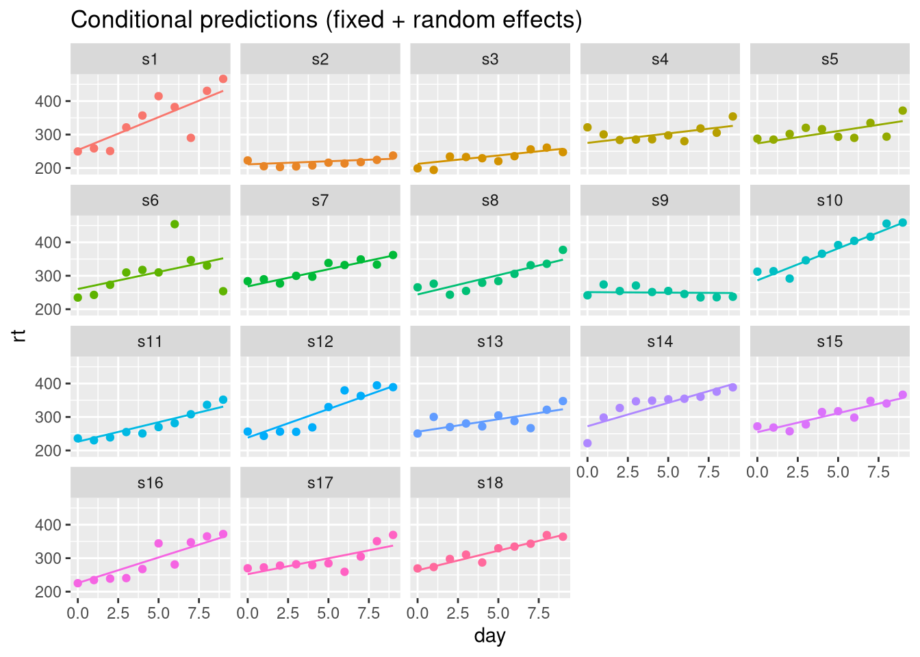
mutate(pvtrt, pred = predict(M7, re.form = NA)) |>
  ggplot(aes(x = day, y = rt, colour = id)) +
  geom_point() +
  geom_line(aes(y = pred)) +
  facet_wrap(~id) +
  theme(legend.position = "none") +
  labs(title = "Marginal predictions (fixed effects only)")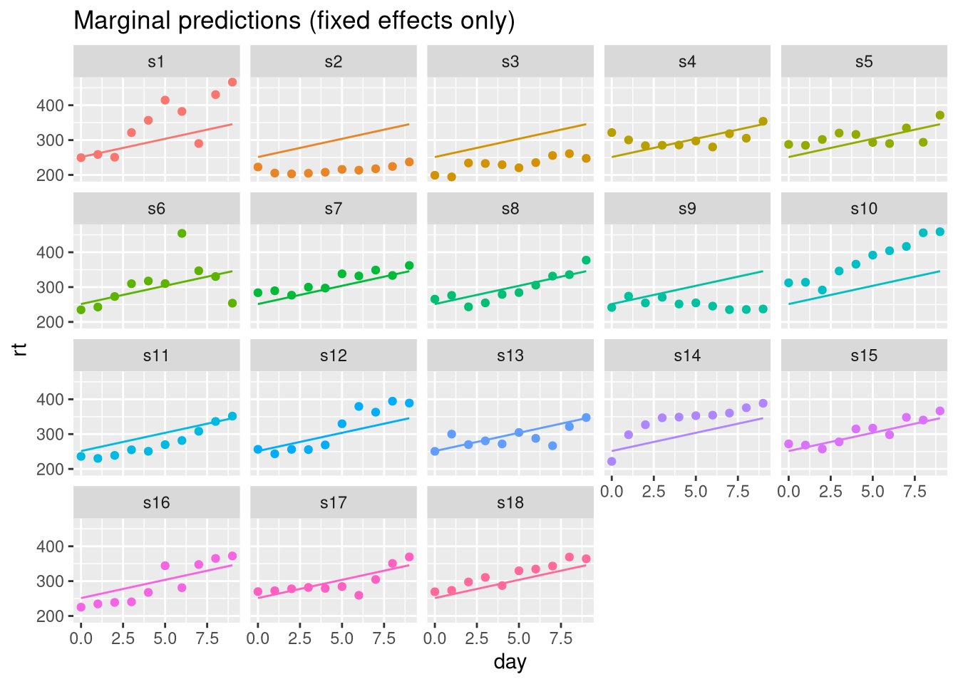
Marginal and conditional R²
Nakagawa and Schielzeth (2013) proposed two \(R^2\) statistics for mixed effects models that mirror this distinction.
Marginal \(R^2\) is the proportion of variance explained by the fixed effects alone. It is analogous to the population-level \(R^2\).
Conditional \(R^2\) is the proportion of variance explained by the full model, including both fixed and random effects. It is the \(R^2\) for the specific subjects in the data.
A simple approximation for both is obtained from the variance of the predicted values.
cond_r2 <- var(predict(M7)) / var(pvtrt$rt)
marg_r2 <- var(predict(M7, re.form = NA)) / var(pvtrt$rt)

cond_r2
[1] 0.7635777marg_r2[1] 0.2864714The gap between conditional and marginal \(R^2\) reflects the contribution of the random effects. When this gap is large, the random effects are capturing substantial individual variability that the fixed effects alone do not.
Computing R² with the performance package
The performance package implements the Nakagawa-Schielzeth method directly, including a more careful treatment of the variance components.
r2_nakagawa(M7)# R2 for Mixed Models
Conditional R2: 0.799
Marginal R2: 0.279The result gives marginal \(R^2\) (fixed effects only) and conditional \(R^2\) (fixed plus random effects).
The Nakagawa-Schielzeth approach partitions the total variance into the variance attributable to fixed effects, variance attributable to random effects, and residual variance, and computes \(R^2\) values from these components directly. This is more principled than the approximation above because it accounts for the variance components estimated by the model rather than the variance of the predictions in the observed data.
Interpreting the values
For the sleep deprivation model, the marginal \(R^2\) reflects how much variance is explained by the population-average effect of days of sleep deprivation. The conditional \(R^2\) additionally captures the fact that individual subjects have consistently higher or lower reaction times and steeper or shallower slopes.
A low marginal but high conditional \(R^2\) indicates that most of the structure in the data is due to individual differences rather than the fixed predictors. A high marginal \(R^2\) indicates that the fixed effects explain much of the variance even before accounting for individual variation.
M8 <- lmer(rt ~ day + (1 | id), data = pvtrt)
r2_nakagawa(M8)
# R2 for Mixed Models
Conditional R2: 0.704
Marginal R2: 0.280The varying-intercepts-only model explains somewhat less variance conditionally than the full model, reflecting the contribution of the random slopes.
Comparison across models
The r2_nakagawa function can be applied to any linear mixed effects model, and comparing the marginal and conditional values across models helps assess the contribution of fixed versus random structure.
M_null <- lmer(rt ~ 1 + (day | id), data = pvtrt)

r2_nakagawa(M_null)
Warning: Random slopes not present as fixed effects. This artificially inflates
the conditional random effect variances.
Respecify the fixed effects structure of your model (add random slopes
as fixed effects).# R2 for Mixed Models
Conditional R2: 0.499
Marginal R2: 0.000r2_nakagawa(M8)# R2 for Mixed Models
Conditional R2: 0.704
Marginal R2: 0.280r2_nakagawa(M7)# R2 for Mixed Models
Conditional R2: 0.799
Marginal R2: 0.279Adding day as a fixed effect increases the marginal \(R^2\). The conditional \(R^2\) is high across all three models because the subject-level random effects capture substantial individual variation regardless of the fixed effects structure.