import torch
import torch.nn as nn

mlp_layer = nn.Linear(784, 128)
cnn_layer  = nn.Conv2d(in_channels=1, out_channels=32, kernel_size=3, padding=1)

sum(p.numel() for p in mlp_layer.parameters())100480Convolutional Neural Networks
We introduce convolutional neural networks as a principled response to the limitations of fully-connected networks on image data. We cover convolutional layers, pooling, and batch normalisation, build a CNN in PyTorch, train it on MNIST, and visualise the learned filters.
A fully-connected layer treats its input as a flat vector. For an image, this means every output unit is connected to every input pixel, which creates two problems.
The first problem is parameter count. A 28×28 greyscale image has 784 pixels. A modest first hidden layer of 128 units requires 784 × 128 = 100,352 weights, plus biases. For a 224×224 colour image — a standard size in computer vision benchmarks — the same layer would require over 19 million weights. This grows quadratically with image resolution and becomes impractical very quickly.
import torch
import torch.nn as nn
mlp_layer = nn.Linear(784, 128)
cnn_layer = nn.Conv2d(in_channels=1, out_channels=32, kernel_size=3, padding=1)
sum(p.numel() for p in mlp_layer.parameters())100480sum(p.numel() for p in cnn_layer.parameters())320The same 128 → 32 transition in representational richness costs over 100,000 parameters in the MLP and 320 in the convolutional layer.
The second problem is that flattening an image discards all spatial structure. A pixel’s value is only meaningful in relation to its neighbours. A fully-connected layer has no mechanism to exploit proximity, and must learn spatial relationships from scratch.
A convolutional layer addresses both problems by replacing the global weight matrix with a set of small, reusable filters. Each filter is a small matrix — typically 3×3 — that slides across the image. At each position it computes a weighted sum of the patch of pixels it covers. The output value at position \((i, j)\) for a single filter \(w\) on a single-channel input \(x\) is:
\[y_{i,j} = \sum_{m=0}^{k-1} \sum_{n=0}^{k-1} x_{i+m,\, j+n} \cdot w_{m,n} + b\]
where \(k\) is the kernel size. This is called local connectivity: each output unit depends only on a small local region of the input.
Because the same filter is applied at every position, the network uses far fewer parameters. This is parameter sharing. It also means the filter learns to detect a feature — an edge, a curve, a texture — regardless of where in the image it appears. This is translation invariance.
The result of sliding one filter across the input is called a feature map. A layer with 32 filters produces 32 feature maps stacked together, one per filter.
Without padding, a 3×3 filter applied to a 28×28 image produces a 26×26 output. Setting padding=1 adds a border of zeros around the input so the output has the same spatial dimensions as the input.
# (batch, channels, height, width)
x = torch.randn(1, 1, 28, 28)     # one 28x28 greyscale image

conv = nn.Conv2d(1, 32, kernel_size=3, padding=1)
out = conv(x)
out.shape                          # (1, 32, 28, 28): 32 feature maps, same spatial size
With a stride of 2, the filter moves two pixels at a time, halving the spatial dimensions.
conv_stride = nn.Conv2d(1, 32, kernel_size=3, stride=2, padding=1)
conv_stride(x).shape              # (1, 32, 14, 14)
Pooling layers reduce spatial dimensions without learnable parameters. Max pooling partitions the feature map into non-overlapping windows and takes the maximum value in each. A 2×2 max pool halves the height and width.
pool = nn.MaxPool2d(kernel_size=2)

x = torch.randn(1, 32, 28, 28)
pool(x).shape                     # (1, 32, 14, 14)
torch.Size([1, 32, 14, 14])Pooling makes representations progressively more compact as depth increases. It also provides a degree of local translation invariance: a feature shifted slightly within a pooling window produces the same output.
Batch normalisation (BatchNorm2d) normalises the activations across a mini-batch, independently for each channel. For a batch of activations with mean \(\mu_B\) and variance \(\sigma_B^2\), the normalised value is:
\[\hat{x} = \frac{x - \mu_B}{\sqrt{\sigma_B^2 + \varepsilon}}\]
Two learnable parameters \(\gamma\) and \(\beta\) then scale and shift the result: \(y = \gamma \hat{x} + \beta\). During training, \(\mu_B\) and \(\sigma_B^2\) are computed from the current mini-batch. During evaluation, running estimates accumulated during training are used instead.
Batch normalisation stabilises training by preventing activations from growing very large or collapsing to zero as they pass through deep networks. It is applied after a convolution and before the activation function.
bn = nn.BatchNorm2d(num_features=32)  # one scale/shift pair per channel

x = torch.randn(16, 32, 14, 14)      # batch of 16, 32 channels
bn(x).shape
torch.Size([16, 32, 14, 14])We now put the pieces together. The architecture applies two rounds of convolution-batchnorm-relu-pool, then classifies with a fully-connected layer. The spatial dimensions evolve as follows: 28×28 → 14×14 → 7×7.
class CNN(nn.Module):
    def __init__(self):
        super().__init__()
        self.conv1 = nn.Conv2d(1, 32, kernel_size=3, padding=1)
        self.bn1   = nn.BatchNorm2d(32)
        self.conv2 = nn.Conv2d(32, 64, kernel_size=3, padding=1)
        self.bn2   = nn.BatchNorm2d(64)
        self.pool  = nn.MaxPool2d(2)
        self.fc    = nn.Linear(64 * 7 * 7, 10)

    def forward(self, x):
        x = self.pool(torch.relu(self.bn1(self.conv1(x))))  # (B, 32, 14, 14)
        x = self.pool(torch.relu(self.bn2(self.conv2(x))))  # (B, 64, 7, 7)
        x = x.flatten(start_dim=1)                          # (B, 3136)
        return self.fc(x)

model = CNN()
model
CNN(
(conv1): Conv2d(1, 32, kernel_size=(3, 3), stride=(1, 1), padding=(1, 1))
(bn1): BatchNorm2d(32, eps=1e-05, momentum=0.1, affine=True, track_running_stats=True)
(conv2): Conv2d(32, 64, kernel_size=(3, 3), stride=(1, 1), padding=(1, 1))
(bn2): BatchNorm2d(64, eps=1e-05, momentum=0.1, affine=True, track_running_stats=True)
(pool): MaxPool2d(kernel_size=2, stride=2, padding=0, dilation=1, ceil_mode=False)
(fc): Linear(in_features=3136, out_features=10, bias=True)
)The flatten call collapses all dimensions except the batch dimension into a single vector, converting the (B, 64, 7, 7) tensor into (B, 3136) before the final linear layer.
sum(p.numel() for p in model.parameters() if p.requires_grad)50378This is far fewer parameters than an MLP of comparable capacity would require.
We reuse the MNIST loaders from the previous session.
from torchvision import datasets, transforms
from torch.utils.data import DataLoader

transform = transforms.ToTensor()
train_data = datasets.MNIST(root='data', train=True,  download=True, transform=transform)
test_data  = datasets.MNIST(root='data', train=False, download=True, transform=transform)

train_loader = DataLoader(train_data, batch_size=64, shuffle=True)
test_loader  = DataLoader(test_data,  batch_size=64)
The images from the DataLoader arrive with shape (B, 1, 28, 28), which is exactly what nn.Conv2d expects. No flattening is needed at the input — the CNN handles the spatial structure directly.
criterion = nn.CrossEntropyLoss()
optimizer = torch.optim.Adam(model.parameters(), lr=1e-3)

losses = []

for epoch in range(5):
    model.train()
    epoch_loss = 0
    for X, y in train_loader:
        optimizer.zero_grad()
        loss = criterion(model(X), y)
        loss.backward()
        optimizer.step()
        epoch_loss += loss.item()
    avg = epoch_loss / len(train_loader)
    losses.append(avg)
    print(f"Epoch {epoch+1}: loss={avg:.4f}")
Epoch 1: loss=0.1245
Epoch 2: loss=0.0507
Epoch 3: loss=0.0386
Epoch 4: loss=0.0302
Epoch 5: loss=0.0250model.eval()
correct = 0
with torch.no_grad():
for X, y in test_loader:
correct += (model(X).argmax(dim=1) == y).sum().item()
print(f"Test accuracy: {correct / len(test_data):.3f}")Test accuracy: 0.990A CNN typically outperforms an MLP of similar parameter count on image tasks, because the inductive bias of local connectivity and parameter sharing fits the structure of images well.
After training, the first convolutional layer has learned 32 filters, each of size 3×3. We can inspect them directly.
import matplotlib.pyplot as plt

filters = model.conv1.weight.data   # shape: (32, 1, 3, 3)

fig, axes = plt.subplots(4, 8, figsize=(10, 5))
for i, ax in enumerate(axes.flat):
    ax.imshow(filters[i, 0], cmap='gray')
    ax.axis('off')
plt.suptitle('Learned filters, conv1')
plt.tight_layout()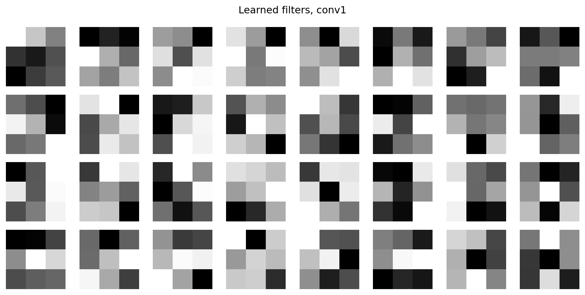
Early filters typically learn low-level features: edges, corners, and gradients in various orientations. The second convolutional layer’s filters operate on the 32 feature maps produced by the first layer and are harder to interpret directly, but they detect higher-level combinations of the earlier features.