We build and train a multilayer perceptron using PyTorch’s nn.Module. The running example is MNIST handwritten digit classification. We first implement the training loop explicitly to see all the moving parts, then replace it with skorch, which provides a scikit-learn compatible interface and reduces the boilerplate considerably.
Defining a network with nn.Module
The standard way to define a network in PyTorch is to subclass nn.Module. The class has two required parts: __init__, which declares the learnable components of the network, and forward, which describes the computation.
import torchimport torch.nn as nnclass MLP(nn.Module):def__init__(self):super().__init__()self.fc1 = nn.Linear(784, 128)self.fc2 = nn.Linear(128, 64)self.fc3 = nn.Linear(64, 10)def forward(self, x): x = torch.relu(self.fc1(x)) x = torch.relu(self.fc2(x))returnself.fc3(x)model = MLP()model
nn.Linear(in_features, out_features) creates a single fully-connected layer. Internally it holds two learnable tensors: a weight matrix \(W\) of shape \((\text{out}, \text{in})\) and a bias vector \(b\) of shape \((\text{out},)\). When called on an input \(x\) of shape \((\text{batch}, \text{in})\), it computes:
\[y = x W^T + b\]
giving an output of shape \((\text{batch}, \text{out})\). Both \(W\) and \(b\) are registered as parameters with requires_grad=True, so gradients flow through them during backward().
nn.Linear(784, 128) therefore creates a \(128 \times 784\) weight matrix. It maps a vector of 784 inputs to a vector of 128 outputs.
Chaining layers
In __init__ we are only declaring the three layers. We are not yet connecting them: fc1, fc2, and fc3 exist as independent objects. The connection between them is specified in forward.
The dimensions must be consistent. The output size of fc1 is 128, so the input size of fc2 must also be 128. The output size of fc2 is 64, so the input size of fc3 must be 64. The network produces 10 outputs, one logit per digit class.
forward
forward defines the computation. It takes an input x and returns an output, passing x through each layer in turn. torch.relu is applied after fc1 and fc2 to introduce non-linearity. No activation is applied after fc3 because the cross-entropy loss expects raw logits.
When you write model(x), PyTorch calls model.forward(x) internally via __call__. The only requirement nn.Module imposes is that you define forward. Everything else, registering parameters, moving the model to a GPU, saving and loading weights, is handled by the base class.
Model parameters
Every nn.Linear layer registers its weight matrix and bias vector as parameters. We can count them.
sum(p.numel() for p in model.parameters() if p.requires_grad)
109386
model.parameters() returns an iterator over all tensors that have requires_grad=True, which is every weight and bias in the network. This is what we pass to the optimizer so that it knows what to update.
nn.Sequential
For straightforward feedforward networks, nn.Sequential avoids writing a class. It takes a list of modules and calls them in order in its own forward method.
Note that here we use nn.ReLU() rather than torch.relu. torch.relu is a plain function; nn.ReLU() is a module, which is what nn.Sequential expects. They compute the same thing.
nn.Sequential is appropriate when data flows straight through from one layer to the next. For anything more complex — skip connections, branching paths, multiple inputs or outputs — you need a full nn.Module subclass.
Loading MNIST
torchvision provides MNIST and other standard datasets. The transform argument applies a preprocessing pipeline to each sample as it is loaded.
transforms.ToTensor() does two things: it converts a PIL image (stored as integers in \([0, 255]\)) to a float tensor in \([0.0, 1.0]\), and it reorders the axes from height-width-channel (HWC, the PIL convention) to channel-height-width (CHW, the PyTorch convention).
The image shape is (1, 28, 28): one channel (greyscale), 28 rows, 28 columns. nn.Linear expects a flat vector, not a 3D tensor, which is why flattening is needed before the first linear layer.
DataLoader
DataLoader wraps a dataset and serves it in mini-batches, handling shuffling and parallel data loading.
We are now ready to train. The explicit training loop below is the standard PyTorch pattern. It is deliberately verbose — the goal is to make every step visible. Later in this session we will use skorch to replace most of this boilerplate with a single call to fit.
First, define the model, the loss function, and the optimizer. The model includes nn.Flatten() as its first layer so that the (batch, 1, 28, 28) images coming from the DataLoader are flattened to (batch, 784) automatically.
The training loop runs for a fixed number of epochs. Within each epoch it iterates over every mini-batch: forward pass, loss, backward pass, parameter update.
losses = []for epoch inrange(5): epoch_loss =0for X, y in train_loader: optimizer.zero_grad() loss = criterion(model(X), y) loss.backward() optimizer.step() epoch_loss += loss.item() avg = epoch_loss /len(train_loader) losses.append(avg)print(f"Epoch {epoch+1}: loss={avg:.4f}")
This is the irreducible core of neural network training in PyTorch. The four lines inside the inner loop — zero_grad, forward pass, backward, step — are always the same regardless of model architecture, dataset, or task.
Evaluation
After training, switch the model to evaluation mode before measuring accuracy. This disables dropout and any other training-specific behaviour. torch.no_grad() suppresses gradient tracking during inference, saving memory and time.
model.eval()correct =0with torch.no_grad():for X, y in test_loader: preds = model(X).argmax(dim=1) correct += (preds == y).sum().item()accuracy = correct /len(test_data)print(f"Test accuracy: {accuracy:.3f}")
Test accuracy: 0.975
argmax(dim=1) picks the class with the highest logit for each sample in the batch.
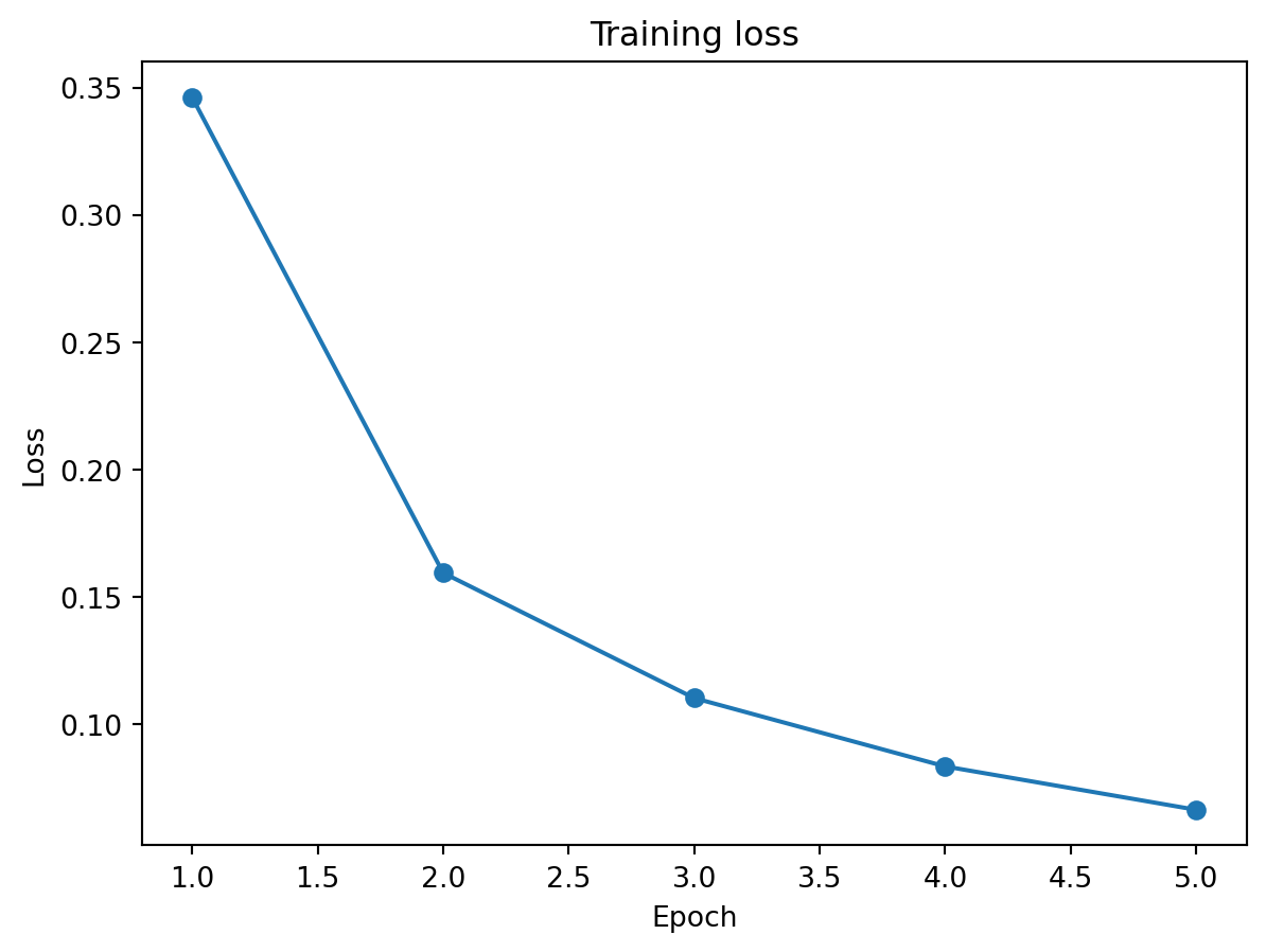
Plotting the loss
import matplotlib.pyplot as pltplt.plot(range(1, 6), losses, marker='o')plt.xlabel('Epoch')plt.ylabel('Loss')plt.title('Training loss')
Text(0.5, 1.0, 'Training loss')
skorch
The explicit loop above works, but it requires writing the same boilerplate every time. skorch wraps PyTorch models in a scikit-learn compatible interface, replacing the manual epoch loop with a single call to fit and printing a formatted training table automatically.
To use skorch we define the network architecture as an nn.Module class and pass the class (not an instance) to NeuralNetClassifier. skorch handles instantiation, the training loop, and evaluation internally.
  epoch    train_loss    valid_acc    valid_loss     dur

-------  ------------  -----------  ------------  ------

      1           nan       0.1044           nan  0.3815

      2           nan       0.1044           nan  0.3776

      3           nan       0.1044           nan  0.3788

      4           nan       0.1044           nan  0.3780

      5           nan       0.1044           nan  0.3752
In a Jupyter environment, please rerun this cell to show the HTML representation or trust the notebook. On GitHub, the HTML representation is unable to render, please try loading this page with nbviewer.org.