Day One, Session One

Introduction to Artificial Neural Networks

Abstract

We implement artificial neurons from scratch using NumPy. We define and plot the common activation functions, then build a simple forward pass through a small two-layer network by hand. The goal is a clear computational picture of what a neural network does before we move to PyTorch in later sessions.

The artificial neuron

An artificial neuron takes a vector of inputs, computes a weighted sum, adds a bias term, and passes the result through an activation function. We can write this in a few lines of NumPy.

import numpy as np

x = np.array([1.5, 2.0, -1.0])   # inputs
w = np.array([0.5, -0.3,  0.8])  # weights
b = 0.1                           # bias

The weighted sum plus bias is called the pre-activation, conventionally written as \(z\).

z = np.dot(x, w) + b
z

np.float64(-0.55)

Passing \(z\) through the sigmoid activation function gives the neuron’s output.

def sigmoid(z):
    return 1 / (1 + np.exp(-z))

sigmoid(z)

np.float64(0.36586440898919936)

Activation functions

The activation function introduces non-linearity into the network. Without it, stacking layers would collapse to a single linear transformation. The three most commonly used functions are sigmoid, tanh, and ReLU.

def tanh(z):
    return np.tanh(z)

def relu(z):
    return np.maximum(0, z)

We can see their shapes by plotting them over a range of inputs.

import matplotlib.pyplot as plt

z = np.linspace(-5, 5, 200)

plt.plot(z, sigmoid(z), label='Sigmoid')
plt.plot(z, tanh(z),    label='Tanh')
plt.plot(z, relu(z),    label='ReLU')
plt.axhline(0, color='k', linewidth=0.5)
plt.legend()
plt.xlabel('z')
plt.title('Activation functions')

Text(0.5, 1.0, 'Activation functions')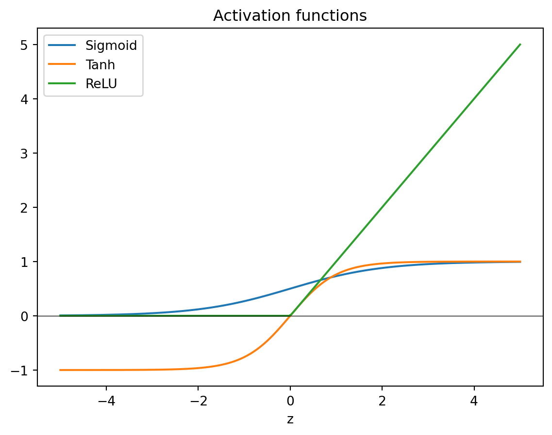

Sigmoid squashes its input to the range \((0, 1)\). Tanh squashes to \((-1, 1)\). ReLU passes positive values unchanged and maps everything negative to zero. In modern networks ReLU and its variants are the default choice for hidden layers because they train faster and avoid the vanishing gradient problem that affects sigmoid and tanh.

We can also write a general neuron that takes the activation as an argument.

def neuron(x, w, b, activation):
    return activation(np.dot(x, w) + b)

x = np.array([1.5, 2.0, -1.0])
w = np.array([0.5, -0.3, 0.8])
b = 0.1

neuron(x, w, b, relu)

np.float64(0.0)

neuron(x, w, b, sigmoid)

np.float64(0.36586440898919936)

A simple network

A network is neurons arranged in layers. Each layer takes the previous layer’s outputs as its inputs. We implement a two-layer network manually to see the computation clearly.

The network has three inputs, four hidden units (using ReLU), and two outputs (using sigmoid). Each layer is defined by a weight matrix and a bias vector.

np.random.seed(42)

W1 = np.random.randn(3, 4) * 0.5  # (inputs, hidden units)
b1 = np.zeros(4)

W2 = np.random.randn(4, 2) * 0.5  # (hidden units, outputs)
b2 = np.zeros(2)

The forward pass computes the output for a single input.

x = np.array([1.5, 2.0, -1.0])

h = relu(x @ W1 + b1)    # hidden layer
h

array([0.37311943, 0.        , 2.29668807, 2.142572  ])

y = sigmoid(h @ W2 + b2)  # output layer
y

array([0.11000484, 0.18107842])

The same logic extends to a batch of inputs by passing a matrix instead of a vector. NumPy’s broadcasting handles the bias addition without any changes to the code.

X = np.array([
    [ 1.5,  2.0, -1.0],
    [-0.5,  1.0,  0.5],
    [ 0.0, -1.5,  2.0],
])

H = relu(X @ W1 + b1)
Y = sigmoid(H @ W2 + b2)
Y

array([[0.11000484, 0.18107842],
       [0.42432891, 0.51636447],
       [0.34992114, 0.44969404]])

Each row of Y is the network’s output for the corresponding row of X. This is exactly what PyTorch does under the hood, at much larger scale and with GPU acceleration.