Poisson regression is the standard model for unbounded count data. This guide covers the Poisson distribution, the log link function, fitting with glm, interpreting coefficients as multiplicative rate ratios, handling exposure via offset terms, and comparing models with deviance and likelihood ratio tests.
The Poisson distribution
The Poisson distribution is a discrete probability distribution over the non-negative integers \(\{0, 1, 2, \ldots\}\). It is parameterised by a single rate parameter \(\lambda > 0\), and its probability mass function is
\[
\Pr(x = k \mid \lambda) = \frac{e^{-\lambda} \lambda^k}{k!}.
\]
A key property is that its mean and variance are both equal to \(\lambda\). This equidispersion property is diagnostic: if the sample variance substantially exceeds the sample mean, a Poisson model may not be appropriate.
Poisson regression
In Poisson regression, we model each count \(y_i\) as a Poisson random variable whose rate \(\lambda_i\) depends on predictors:
The log link ensures \(\lambda_i > 0\) regardless of the predictor values. Equivalently, \(\lambda_i = \exp(\beta_0 + \sum_k \beta_k x_{ki})\).
Fitting with glm
The DoctorAUS.csv dataset records the number of visits to a doctor in a fixed period along with predictors including age, sex, and income.
doctor_df <-read_csv("https://raw.githubusercontent.com/mark-andrews/iglmr24/main/data/DoctorAUS.csv") |>mutate(age = age *100)
New names:
Rows: 5190 Columns: 16
── Column specification
──────────────────────────────────────────────────────── Delimiter: "," chr
(2): insurance, chcond dbl (14): ...1, sex, age, income, illness, actdays,
hscore, doctorco, nondoc...
ℹ Use `spec()` to retrieve the full column specification for this data. ℹ
Specify the column types or set `show_col_types = FALSE` to quiet this message.
• `` -> `...1`
Call:
glm(formula = doctorco ~ age, family = poisson(link = "log"),
    data = doctor_df)

Coefficients:
             Estimate Std. Error z value Pr(>|z|)
(Intercept) -1.879438   0.062482  -30.08   <2e-16 ***
age          0.015488   0.001206   12.84   <2e-16 ***
---
Signif. codes:  0 '***' 0.001 '**' 0.01 '*' 0.05 '.' 0.1 ' ' 1

(Dispersion parameter for poisson family taken to be 1)

    Null deviance: 5634.8  on 5189  degrees of freedom
Residual deviance: 5470.0  on 5188  degrees of freedom
AIC: 7805.6

Number of Fisher Scoring iterations: 6
confint.default(M_10)
                  2.5 %      97.5 %
(Intercept) -2.00190130 -1.75697545
age          0.01312404  0.01785148
Interpreting coefficients
On the log scale, a one-unit increase in a predictor adds \(\beta_k\) to \(\log(\lambda)\). On the original count scale, this corresponds to multiplying\(\lambda\) by \(e^{\beta_k}\). This multiplicative interpretation makes \(e^{\beta_k}\) the natural summary: it is the factor by which the expected count changes for a one-unit increase in the predictor.
estimates <-coef(M_10)exp(estimates["age"]) # multiplicative change per unit increase in age
     age
1.015608
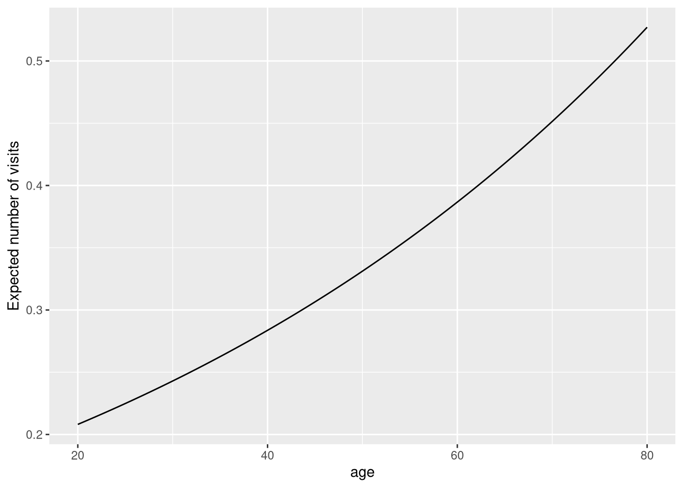
# predicted average doctor visits at ages 25 and 75exp(estimates[1] + estimates[2] *25)
(Intercept)
  0.2248674
exp(estimates[1] + estimates[2] *75)
(Intercept)
  0.4877968
Predictions over a range of ages:
doctor_new <-tibble(age =seq(20, 80))add_predictions(doctor_new, M_10, type ="response") |>ggplot(aes(x = age, y = pred)) +geom_line() +labs(y ="Expected number of visits")
Model comparison
A model with additional predictors:
M_12 <-glm(doctorco ~ sex + age + income,data = doctor_df,family =poisson(link ="log"))anova(M_10, M_12, test ="Chisq")
Analysis of Deviance Table

Model 1: doctorco ~ age
Model 2: doctorco ~ sex + age + income
  Resid. Df Resid. Dev Df Deviance  Pr(>Chi)
1      5188     5470.0
2      5186     5434.9  2   35.129 2.354e-08 ***
---
Signif. codes:  0 '***' 0.001 '**' 0.01 '*' 0.05 '.' 0.1 ' ' 1
Exposure and offset terms
When the period of observation varies across individuals — for example some people are observed for six months and others for a year — the counts are not directly comparable. We adjust by including the log of the exposure time as a fixed offset in the linear predictor:
New names:
Rows: 64 Columns: 6
── Column specification
──────────────────────────────────────────────────────── Delimiter: "," chr
(2): Group, Age dbl (4): ...1, District, Holders, Claims
ℹ Use `spec()` to retrieve the full column specification for this data. ℹ
Specify the column types or set `show_col_types = FALSE` to quiet this message.
• `` -> `...1`
M_ins <-glm(Claims ~ District + Group + Age +offset(log(Holders)),data = insur_df,family = poisson)summary(M_ins)
Call:
glm(formula = Claims ~ District + Group + Age + offset(log(Holders)),
    family = poisson, data = insur_df)

Coefficients:
            Estimate Std. Error z value Pr(>|z|)
(Intercept) -1.82174    0.07679 -23.724  < 2e-16 ***
District2    0.02587    0.04302   0.601 0.547597
District3    0.03852    0.05051   0.763 0.445657
District4    0.23421    0.06167   3.798 0.000146 ***
Group>2l     0.56341    0.07232   7.791 6.65e-15 ***
Group1-1.5l  0.16134    0.05053   3.193 0.001409 **
Group1.5-2l  0.39281    0.05500   7.142 9.18e-13 ***
Age>35      -0.53667    0.06996  -7.672 1.70e-14 ***
Age25-29    -0.19101    0.08286  -2.305 0.021149 *
Age30-35    -0.34495    0.08137  -4.239 2.24e-05 ***
---
Signif. codes:  0 '***' 0.001 '**' 0.01 '*' 0.05 '.' 0.1 ' ' 1

(Dispersion parameter for poisson family taken to be 1)

    Null deviance: 236.26  on 63  degrees of freedom
Residual deviance:  51.42  on 54  degrees of freedom
AIC: 388.74

Number of Fisher Scoring iterations: 4
The coefficients now refer to the log rate (claims per holder) rather than the raw count.