Binomial Logistic Regression

Author

Mark Andrews

Abstract

When count data have a known upper bound — the number of successes out of a fixed number of trials — the binomial logistic regression model is appropriate. This guide covers the binomial distribution, the relationship to binary logistic regression, and practical fitting with glm using the cbind response syntax.

Bounded count data

Poisson regression models unbounded counts — in principle, any non-negative integer is possible. But some counting situations have a natural maximum: the number of questions answered correctly out of a fixed test, the number of items approved out of a batch of known size, or the number of putts made out of a fixed number of attempts. In these cases, the binomial distribution is the appropriate likelihood.

The binomial logistic regression model

For observation \(i\), suppose \(y_i\) is the number of successes in \(n_i\) independent trials, where each trial succeeds with probability \(\theta_i\). The model is

\[ \begin{aligned} y_i &\sim \mathrm{Binomial}(n_i, \theta_i),\\ \mathrm{logit}(\theta_i) &= \beta_0 + \sum_k \beta_k x_{ki}. \end{aligned} \]

The same logit link and linear predictor from binary logistic regression appear here. When \(n_i = 1\) for all observations, the binomial distribution reduces to the Bernoulli distribution and this model becomes ordinary binary logistic regression.

Fitting with glm

The golf_putts.csv dataset records the number of successful putts and attempts at each distance from the hole.

golf_df <- read_csv("https://raw.githubusercontent.com/mark-andrews/iglmr24/main/data/golf_putts.csv") |>
  mutate(
    failure = attempts - success,
    p = success / attempts
  )

Rows: 19 Columns: 3
── Column specification ────────────────────────────────────────────────────────
Delimiter: ","
dbl (3): distance, attempts, success

ℹ Use `spec()` to retrieve the full column specification for this data.
ℹ Specify the column types or set `show_col_types = FALSE` to quiet this message.

golf_df

# A tibble: 19 × 5
   distance attempts success failure     p
      <dbl>    <dbl>   <dbl>   <dbl> <dbl>
 1        2     1443    1346      97 0.933
 2        3      694     577     117 0.831
 3        4      455     337     118 0.741
 4        5      353     208     145 0.589
 5        6      272     149     123 0.548
 6        7      256     136     120 0.531
 7        8      240     111     129 0.462
 8        9      217      69     148 0.318
 9       10      200      67     133 0.335
10       11      237      75     162 0.316
11       12      202      52     150 0.257
12       13      192      46     146 0.240
13       14      174      54     120 0.310
14       15      167      28     139 0.168
15       16      201      27     174 0.134
16       17      195      31     164 0.159
17       18      191      33     158 0.173
18       19      147      20     127 0.136
19       20      152      24     128 0.158

To specify the binomial response, we use cbind(successes, failures):

M_bin <- glm(cbind(success, failure) ~ distance,
             family = binomial(link = "logit"),
             data = golf_df)
summary(M_bin)


Call:
glm(formula = cbind(success, failure) ~ distance, family = binomial(link = "logit"), 
    data = golf_df)

Coefficients:
             Estimate Std. Error z value Pr(>|z|)    
(Intercept)  2.231211   0.058463   38.16   <2e-16 ***
distance    -0.255692   0.006691  -38.22   <2e-16 ***
---
Signif. codes:  0 '***' 0.001 '**' 0.01 '*' 0.05 '.' 0.1 ' ' 1

(Dispersion parameter for binomial family taken to be 1)

    Null deviance: 2411.10  on 18  degrees of freedom
Residual deviance:  255.34  on 17  degrees of freedom
AIC: 365.92

Number of Fisher Scoring iterations: 4

Interpreting and predicting

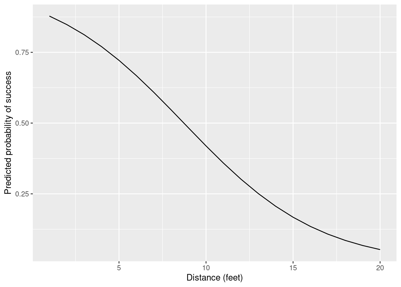
The coefficient for distance is on the log-odds scale. A negative coefficient means that the log odds of success decrease as distance increases, which is what we expect for golf putting.

Predicted probabilities over a range of distances:

golf_new <- tibble(distance = seq(1, 20))
add_predictions(golf_new, M_bin, type = "response") |>
  ggplot(aes(x = distance, y = pred)) +
  geom_line() +
  labs(y = "Predicted probability of success",
       x = "Distance (feet)")

Relationship to binary logistic regression

The binomial logistic regression model reduces exactly to binary logistic regression when every \(n_i = 1\). In that case, cbind(success, failure) has rows of the form (1, 0) or (0, 1), and the model is identical to fitting glm(y ~ x, family = binomial) where y is the binary outcome. The two are the same model; the binomial is simply the more general form.