Multilayer Perceptrons with torch

Abstract

We build and train a multilayer perceptron using torch’s nn_module. The running example is MNIST handwritten digit classification. We first implement the training loop explicitly to see all the moving parts, then replace it with luz, which provides a high-level training interface and reduces the boilerplate considerably.

Defining a network with nn_module

The standard way to define a network in torch for R is to use nn_module. The function takes two key components: initialize, which declares the learnable components of the network, and forward, which describes the computation.

library(torch)

MLP <- nn_module(
  initialize = function() {
    self$fc1 <- nn_linear(784, 128)
    self$fc2 <- nn_linear(128, 64)
    self$fc3 <- nn_linear(64, 10)
  },
  forward = function(x) {
    x <- nnf_relu(self$fc1(x))
    x <- nnf_relu(self$fc2(x))
    self$fc3(x)
  }
)

model <- MLP()
model

An `nn_module` containing 109,386 parameters.

── Modules ─────────────────────────────────────────────────────────────────────
• fc1: <nn_linear> #100,480 parameters
• fc2: <nn_linear> #8,256 parameters
• fc3: <nn_linear> #650 parameters

nn_linear

nn_linear(in_features, out_features) creates a single fully-connected layer. Internally it holds two learnable tensors: a weight matrix \(W\) of shape \((\text{out}, \text{in})\) and a bias vector \(b\) of shape \((\text{out},)\). When called on an input \(x\) of shape \((\text{batch}, \text{in})\), it computes:

\[y = x W^T + b\]

giving an output of shape \((\text{batch}, \text{out})\).

Chaining layers

In initialize we are only declaring the three layers. The connection between them is specified in forward. The dimensions must be consistent: the output size of fc1 is 128, so the input size of fc2 must also be 128, and so on. The network produces 10 outputs, one logit per digit class.

forward

forward defines the computation. nnf_relu is applied after fc1 and fc2 to introduce non-linearity. No activation is applied after fc3 because the cross-entropy loss expects raw logits.

Model parameters

Every nn_linear layer registers its weight matrix and bias vector as parameters. We can count them.

sum(sapply(model$parameters, function(p) prod(p$shape)))

[1] 109386

model$parameters returns a list of all learnable tensors in the network. This is what we pass to the optimizer so that it knows what to update.

nn_sequential

For straightforward feedforward networks, nn_sequential avoids writing a full nn_module. It takes a sequence of modules and calls them in order.

model <- nn_sequential(
  nn_flatten(),
  nn_linear(784, 128),
  nn_relu(),
  nn_linear(128, 64),
  nn_relu(),
  nn_linear(64, 10)
)

nn_relu() is a module, which is what nn_sequential expects. nn_flatten() collapses all dimensions except the batch dimension into a single vector.

nn_sequential is appropriate when data flows straight through from one layer to the next. For anything more complex — skip connections, branching paths, multiple inputs or outputs — you need a full nn_module.

Loading MNIST

torchvision provides MNIST and other standard datasets. The transform argument applies a preprocessing function to each sample as it is loaded. transform_to_tensor converts each image to a float tensor with values in \([0.0, 1.0]\).

library(torchvision)

train_data <- mnist_dataset(
  root      = "data",
  train     = TRUE,
  download  = TRUE,
  transform = transform_to_tensor
)

Split "train" of dataset <mnist> (~12 MB) will be downloaded and processed if
not already available.
<mnist> dataset loaded with 60000 images across 10 classes.

test_data <- mnist_dataset(
  root      = "data",
  train     = FALSE,
  download  = TRUE,
  transform = transform_to_tensor
)

Split "test" of dataset <mnist> (~12 MB) will be downloaded and processed if
not already available.
<mnist> dataset loaded with 10000 images across 10 classes.

c(length(train_data), length(test_data))

[1] 60000 10000

Each sample is a list of (image, label).

sample <- train_data[1]
img   <- sample[[1]]
label <- sample[[2]]
img$shape

[1]  1 28 28

label

[1] 6

The image shape is [1, 28, 28]: one channel (greyscale), 28 rows, 28 columns. nn_linear expects a flat vector, not a 3D tensor, which is why nn_flatten is needed before the first linear layer.

dataloader

dataloader wraps a dataset and serves it in mini-batches, handling shuffling and parallel data loading.

train_loader <- dataloader(train_data, batch_size = 64, shuffle = TRUE)
test_loader  <- dataloader(test_data,  batch_size = 64)

Each iteration yields a list of (images, labels) where images has shape [batch_size, 28, 28]. The channel dimension (size 1 for greyscale) is omitted by the default batch collation in torch for R. The nn_flatten() layer at the start of the network handles this correctly, flattening [B, 28, 28] to [B, 784].

b <- dataloader_make_iter(train_loader)$.next()
b[[1]]$shape

[1] 64  1 28 28

b[[2]]$shape

[1] 64

Training loop

We are now ready to train. The explicit training loop below is the standard torch pattern. It is deliberately verbose — the goal is to make every step visible. Later in this session we will use luz to replace most of this boilerplate.

First, define the model, the loss function, and the optimizer. The model includes nn_flatten() as its first layer so that the [batch, 1, 28, 28] images coming from the dataloader are flattened to [batch, 784] automatically.

model <- nn_sequential(
  nn_flatten(),
  nn_linear(784, 128),
  nn_relu(),
  nn_linear(128, 10)
)

criterion <- nn_cross_entropy_loss()
optimizer <- optim_adam(model$parameters, lr = 1e-3)

The training loop runs for a fixed number of epochs. Within each epoch it iterates over every mini-batch: forward pass, loss, backward pass, parameter update.

losses <- c()

for (epoch in seq_len(5)) {
  epoch_loss <- 0
  coro::loop(for (batch in train_loader) {
    optimizer$zero_grad()
    loss <- criterion(model(batch[[1]]), batch[[2]])
    loss$backward()
    optimizer$step()
    epoch_loss <- epoch_loss + loss$item()
  })
  avg <- epoch_loss / length(train_loader)
  losses <- c(losses, avg)
  cat(sprintf("Epoch %d: loss=%.4f\n", epoch, avg))
}

Epoch 1: loss=0.3477
Epoch 2: loss=0.1564
Epoch 3: loss=0.1088
Epoch 4: loss=0.0826
Epoch 5: loss=0.0655

This is the irreducible core of neural network training in torch. The four lines inside the inner loop — zero_grad, forward pass, backward, step — are always the same regardless of model architecture, dataset, or task.

Evaluation

After training, switch the model to evaluation mode before measuring accuracy. This disables dropout and any other training-specific behaviour. with_no_grad suppresses gradient tracking during inference, saving memory and time.

model$eval()
correct <- 0

with_no_grad({
  coro::loop(for (batch in test_loader) {
    preds <- model(batch[[1]])$argmax(dim = 2)
    correct <- correct + (preds == batch[[2]])$sum()$item()
  })
})

accuracy <- correct / length(test_data)
cat(sprintf("Test accuracy: %.3f\n", accuracy))

Test accuracy: 0.973

argmax(dim = 2) picks the class with the highest logit for each sample in the batch. In torch for R, dimensions are 1-indexed, so dim = 2 refers to the class dimension of the [batch, classes] output tensor.

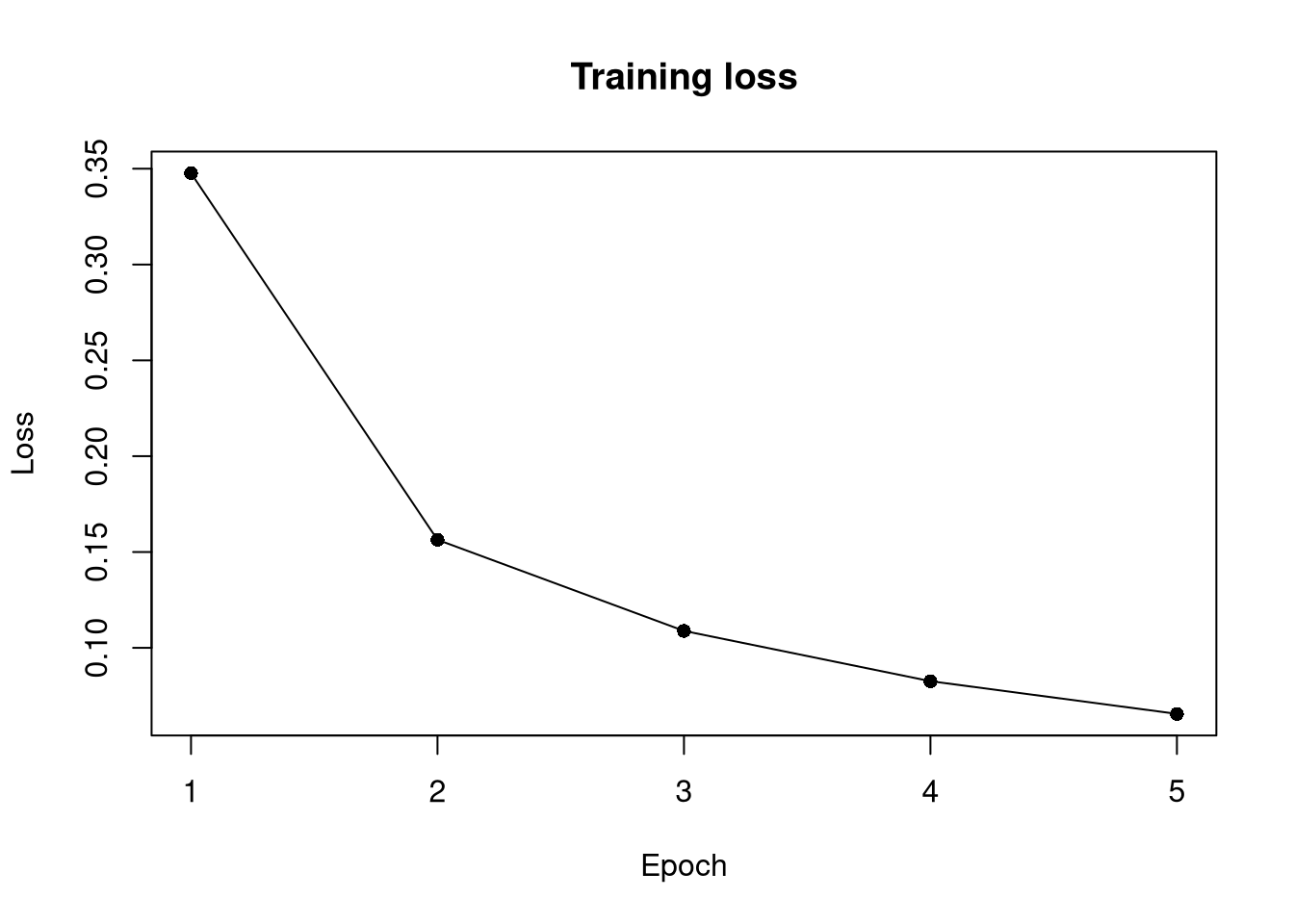
Plotting the loss

plot(seq_along(losses), losses, type = "o", pch = 16,
     xlab = "Epoch", ylab = "Loss", main = "Training loss")

luz

The explicit loop above works, but it requires writing the same boilerplate every time. luz wraps torch models in a high-level training interface, replacing the manual epoch loop with a single call to fit and printing a formatted training table automatically.

To use luz we define the network architecture as an nn_module and pass the class (not an instance) to setup. luz handles the training loop, evaluation, and metric computation internally.

library(luz)

SmallMLP <- nn_module(
  initialize = function() {
    self$net <- nn_sequential(
      nn_linear(784, 128),
      nn_relu(),
      nn_linear(128, 10)
    )
  },
  forward = function(x) self$net(x)
)

The data must be provided via dataloaders. We prepare flat tensors from the raw MNIST arrays. train_data$data holds the images as a plain R array; torch_tensor() converts it to a tensor before further operations.

X_train <- torch_tensor(train_data$data)$float()$reshape(c(-1L, 784L)) / 255
y_train <- torch_tensor(train_data$targets, dtype = torch_long())

X_test <- torch_tensor(test_data$data)$float()$reshape(c(-1L, 784L)) / 255
y_test <- torch_tensor(test_data$targets, dtype = torch_long())

flat_train <- tensor_dataset(X_train, y_train)
flat_test  <- tensor_dataset(X_test, y_test)

flat_train_loader <- dataloader(flat_train, batch_size = 64, shuffle = TRUE)
flat_test_loader  <- dataloader(flat_test,  batch_size = 64)

fitted <- SmallMLP %>%
  setup(
    loss      = nn_cross_entropy_loss(),
    optimizer = optim_adam,
    metrics   = list(luz_metric_accuracy())
  ) %>%
  fit(
    flat_train_loader,
    epochs     = 5,
    valid_data = flat_test_loader
  )

evaluate(fitted, flat_test_loader)

A `luz_module_evaluation`
── Results ─────────────────────────────────────────────────────────────────────
loss: 0.0896
acc: 0.9723

Because luz provides a consistent interface, switching architectures, loss functions, or optimizers requires only changing the relevant arguments to setup.