Introduction to Artificial Neural Networks

Author

Mark Andrews

Abstract

We introduce torch as the computing environment for the course, then use it to build and run a neural network from first principles. Working through the artificial neuron, the common activation functions, and a two-layer forward pass gives a clear and concrete picture of what a neural network computes. We then define the same network as an nn_module, the standard way to build networks in torch.

torch

torch is the primary tool we use throughout this course. It is a library for n-dimensional array computation — the R equivalent of NumPy or MATLAB — with two additional capabilities built in from the start: operations can run on a GPU, and torch can automatically differentiate through any sequence of operations.

library(torch)

x <- torch_tensor(c(1.5, 2.0, -1.0))
x

torch_tensor
 1.5000
 2.0000
-1.0000
[ CPUFloatType{3} ]

x$shape

[1] 3

x$dtype

torch_Float

Tensors and plain R vectors convert to one another cheaply.

as.numeric(x)

[1]  1.5  2.0 -1.0

The standard arithmetic operations work element-wise.

x + x

torch_tensor
 3
 4
-2
[ CPUFloatType{3} ]

x * 2

torch_tensor
 3
 4
-2
[ CPUFloatType{3} ]

x^2

torch_tensor
 2.2500
 4.0000
 1.0000
[ CPUFloatType{3} ]

The key operation for neural networks is the dot product (inner product) of two vectors and the multiplication of matrices.

w <- torch_tensor(c(0.5, -0.3, 0.8))

torch_dot(x, w)

torch_tensor
-0.6500000357627869
[ CPUFloatType{} ]

For matrices, $mv() multiplies a matrix by a vector and $mm() multiplies two matrices.

W <- torch_randn(4, 3)   # 4 rows, 3 columns
W$mv(x)                  # matrix times vector: shape (4,)

torch_tensor
 0.0770
 3.1143
-2.7311
 2.3024
[ CPUFloatType{4} ]

This is the core operation in a neural network layer.

The artificial neuron

An artificial neuron takes a vector of inputs $\mathbf{x}$, computes a weighted sum $\mathbf{w} \cdot \mathbf{x} + b$, and passes the result through an activation function. The weighted sum before the activation is called the pre-activation, conventionally written $z$.

\[z = \mathbf{w} \cdot \mathbf{x} + b = \sum_i w_i x_i + b\]

x <- torch_tensor(c(1.5, 2.0, -1.0))
w <- torch_tensor(c(0.5, -0.3,  0.8))
b <- torch_tensor(0.1)

z <- torch_dot(w, x) + b
z

torch_tensor
-0.5500
[ CPUFloatType{1} ]

Passing $z$ through the sigmoid function gives a number between 0 and 1.

torch_sigmoid(z)

torch_tensor
 0.3659
[ CPUFloatType{1} ]

Activation functions

The activation function is what gives neural networks their power. Without it, stacking layers of weighted sums would collapse to a single linear transformation, no matter how many layers were used. A non-linear activation between layers breaks that collapse and allows the network to approximate any function.

torch provides the common activation functions directly.

z_ex <- torch_tensor(1.5)

torch_sigmoid(z_ex)     # output in (0, 1): historically used in output layers

torch_tensor
 0.8176
[ CPUFloatType{1} ]

torch_tanh(z_ex)        # output in (-1, 1)

torch_tensor
 0.9051
[ CPUFloatType{1} ]

nnf_relu(z_ex)          # max(0, z): the standard choice for hidden layers

torch_tensor
 1.5000
[ CPUFloatType{1} ]

nnf_gelu(z_ex)          # smooth approximation to ReLU: common in transformers

torch_tensor
 1.3998
[ CPUFloatType{1} ]

Sigmoid squashes inputs to $(0, 1)$. Tanh squashes to $(-1, 1)$. ReLU passes positive values unchanged and sets negative values to zero. GELU is a smooth version of ReLU that has become standard in transformer-based models.

We can see their shapes by plotting them over a range of inputs.

z_range <- torch_linspace(-5, 5, 200)

plot(as.numeric(z_range), as.numeric(torch_sigmoid(z_range)),
     type = "l", col = "steelblue", lwd = 2,
     ylim = c(-1.1, 1.1), xlab = "z", ylab = "",
     main = "Activation functions")
lines(as.numeric(z_range), as.numeric(torch_tanh(z_range)),
      col = "firebrick", lwd = 2)
lines(as.numeric(z_range), as.numeric(nnf_relu(z_range)),
      col = "darkgreen", lwd = 2)
lines(as.numeric(z_range), as.numeric(nnf_gelu(z_range)),
      col = "darkorange", lwd = 2, lty = 2)
abline(h = 0, col = "grey70", lwd = 0.5)
legend("topleft",
       legend = c("Sigmoid", "Tanh", "ReLU", "GELU"),
       col    = c("steelblue", "firebrick", "darkgreen", "darkorange"),
       lty    = c(1, 1, 1, 2), lwd = 2)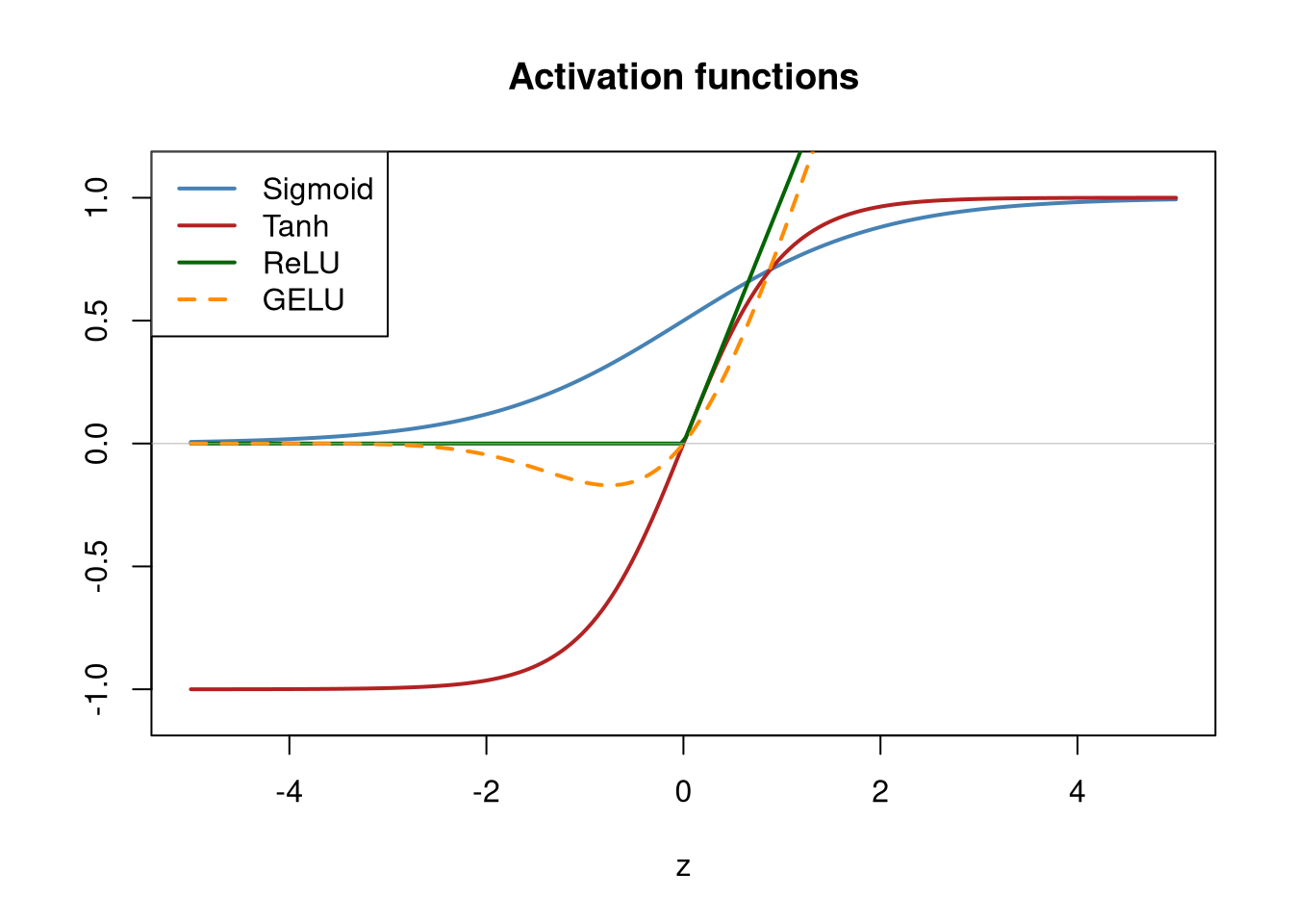

ReLU and GELU are the dominant choices for hidden layers in modern networks. Sigmoid and tanh still appear in specific contexts — sigmoid at the output layer of a binary classifier, tanh inside recurrent cells — but they are rarely used in hidden layers of deep networks because their gradients saturate (approach zero) for large inputs, which slows learning.

A two-layer network

A network is neurons arranged in layers. The outputs of one layer become the inputs to the next. For a single input vector $\mathbf{x}$, a layer with weight matrix $W$ and bias vector $\mathbf{b}$ computes:

\[\mathbf{h} = f(W \mathbf{x} + \mathbf{b})\]

where $f$ is the activation function applied element-wise.

We build a two-layer network with three inputs, four hidden units (ReLU activation), and two outputs.

torch_manual_seed(42)

W1 <- torch_randn(4, 3)   # weight matrix: 4 hidden units, 3 inputs
b1 <- torch_zeros(4)

W2 <- torch_randn(2, 4)   # weight matrix: 2 outputs, 4 hidden units
b2 <- torch_zeros(2)

The forward pass for a single input:

x_in <- torch_tensor(c(1.0, 0.5, -1.0))

h   <- nnf_relu(W1$mv(x_in) + b1)   # hidden layer: shape (4,)
out <- W2$mv(h) + b2                 # output: shape (2,)

h

torch_tensor
 0.1666
 0.0000
 1.4275
 0.0000
[ CPUFloatType{4} ]

out

torch_tensor
-1.2268
-0.8730
[ CPUFloatType{2} ]

$mv() is matrix-times-vector. The hidden layer computes four weighted sums (one per hidden unit), applies ReLU, and produces four activations. The output layer takes those four activations and produces two output values.

For a batch of inputs, $mm() replaces $mv(). The weight matrix convention swaps: inputs are rows, so $mm() needs x on the left.

X <- torch_randn(8, 3)              # 8 inputs, 3 features each

H   <- nnf_relu(X$mm(W1$t()) + b1) # shape (8, 4): 8 hidden vectors
Out <- H$mm(W2$t()) + b2            # shape (8, 2): 8 output vectors

Out$shape

[1] 8 2

$t() transposes the weight matrix so the dimensions align: $W$ is $(d_\text{out} \times d_\text{in})$, and the batch input $X$ is $(n \times d_\text{in})$, so $X W^T$ gives $(n \times d_\text{out})$.

Defining networks with nn_module

Writing out weight matrices and forward pass arithmetic by hand is instructive, but in practice you would never do it. torch provides nn_module to define networks as reusable objects with named layers.

The same two-layer network as an nn_module:

TwoLayerNet <- nn_module(
  initialize = function(n_input, n_hidden, n_output) {
    self$layer1 <- nn_linear(n_input,  n_hidden)
    self$layer2 <- nn_linear(n_hidden, n_output)
  },
  forward = function(x) {
    h <- nnf_relu(self$layer1(x))
    self$layer2(h)
  }
)

model <- TwoLayerNet(n_input = 3, n_hidden = 4, n_output = 2)
model

An `nn_module` containing 26 parameters.

── Modules ─────────────────────────────────────────────────────────────────────
• layer1: <nn_linear> #16 parameters
• layer2: <nn_linear> #10 parameters

nn_linear(in, out) is a layer that holds a weight matrix and bias vector and applies $W\mathbf{x} + \mathbf{b}$ when called. The initialize function declares the layers; forward describes how data flows through them.

A forward pass now looks like any function call.

x_single <- torch_tensor(c(1.0, 0.5, -1.0))
model(x_single)

torch_tensor
-0.1046
-0.3103
[ CPUFloatType{2} ][ grad_fn = <ViewBackward0> ]

X_batch <- torch_randn(8, 3)
model(X_batch)$shape    # (8, 2): one output vector per input

[1] 8 2

The weights are random at this point — the network is not trained and the outputs are meaningless. The next topic covers how training works: how to measure how wrong the output is, how to compute the gradient of that error with respect to every weight, and how to adjust all the weights to make the error smaller.