Inference in the Bernoulli Model

Abstract

A complete treatment of Bayesian inference using the analytically tractable Bernoulli model. We visualise how the posterior combines prior and likelihood, compute point and interval estimates, and introduce the concepts of credible intervals and highest posterior density intervals.

library(priorexposure)
library(tidyverse)

Visualising the posterior

Because the beta prior is conjugate to the binomial likelihood, we can compute the posterior analytically. With \(m = 139\) successes in \(n = 250\) trials and a \(\text{Beta}(3, 5)\) prior, the posterior is \(\text{Beta}(142, 116)\). The bernoulli_posterior_plot function draws all three distributions together, making it easy to see how the data update the prior.

n <- 250
m <- 139
alpha <- 3
beta <- 5

bernoulli_posterior_plot(n, m, alpha = alpha, beta = beta)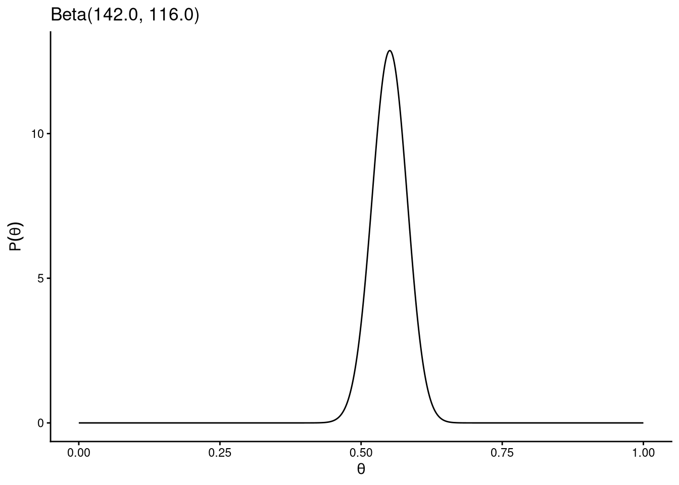

The posterior sits between the prior and the likelihood, pulled toward the likelihood by the weight of the data. With 250 observations the data dominate: the prior has relatively little influence.

Changing to a uniform prior illustrates this directly.

bernoulli_posterior_plot(n, m, alpha = 1, beta = 1)

With a flat prior the posterior is essentially the normalised likelihood. The two plots look almost identical because 250 observations are enough to swamp any weak prior.

Point estimation

The posterior distribution contains all the information the data provide about \(\theta\). Point estimates are summaries of this distribution. The most common choices are the posterior mean and the maximum a posteriori (MAP) estimate, which is the mode of the posterior.

For a \(\text{Beta}(\alpha^*, \beta^*)\) posterior, the mean is \(\alpha^*/(\alpha^* + \beta^*)\) and the mode is \((\alpha^* - 1)/(\alpha^* + \beta^* - 2)\). Both converge to the MLE \(m/n\) as the data dominate the prior.

bernoulli_posterior_summary(n, m, alpha = 1, beta = 1)

$mean
[1] 0.5555556

$var
[1] 0.000975943

$sd
[1] 0.03124009

$mode
[1] 0.556

$qi
[1] 0.4939610 0.6163147

bernoulli_posterior_summary(n, m, alpha = 3, beta = 5)

$mean
[1] 0.5503876

$var
[1] 0.0009554482

$sd
[1] 0.03091033

$mode
[1] 0.5507812

$qi
[1] 0.4894851 0.6105500

Credible intervals

A posterior credible interval is a range of \(\theta\) values that contains a specified fraction of the posterior probability mass. A 95% credible interval contains 95% of the posterior, meaning we assign 95% probability to \(\theta\) lying in that range. This is a direct probability statement about the parameter, which is exactly the kind of statement frequentist confidence intervals cannot make.

Quantile-based intervals

The most straightforward credible interval takes the 2.5th and 97.5th percentiles of the posterior distribution.

qbeta(0.025, m + 1, n - m + 1) # lower bound with uniform prior

[1] 0.493961

qbeta(0.975, m + 1, n - m + 1) # upper bound

[1] 0.6163147

Highest posterior density intervals

The highest posterior density (HPD) interval is the shortest interval containing the specified probability mass. For a unimodal symmetric posterior the quantile and HPD intervals coincide, but for skewed or multimodal posteriors they differ. The HPD interval is generally preferred because it is the most compact region consistent with the data.

get_beta_hpd(m + 1, n - m + 1)

$lb
[1] 0.4943

$ub
[1] 0.6166

$p_star
[1] 1.887

Monte Carlo as a preview of MCMC

We have been computing posterior quantities analytically because the beta posterior has a known closed form. For most realistic models no such closed form exists. The standard solution is to draw random samples from the posterior and use those samples to approximate any quantity of interest.

As a preview, we can sample from a normal distribution and use the samples to estimate probabilities exactly as we will later use MCMC samples from complex posteriors.

set.seed(41)
x <- rnorm(n = 1e6, mean = 100, sd = 15)

mean(x)

[1] 100.0219

sd(x)

[1] 14.99414

pnorm(130, mean = 100, sd = 15) # exact probability

[1] 0.9772499

mean(x <= 130) # Monte Carlo approximation

[1] 0.977204

With one million samples the approximation is accurate to four decimal places. MCMC does the same thing for posterior distributions that have no closed form: it generates samples from the posterior, and we use those samples to compute means, intervals, and any other summary we need.