Bayes’ Rule and the Bernoulli Model

Abstract

We derive Bayes’ rule from the product rule of probability and apply it to the Bernoulli model. Using the priorexposure package we visualise the likelihood function and explore how the beta distribution family represents different prior beliefs about the unknown parameter.

library(priorexposure)
library(tidyverse)

Deriving Bayes’ rule

Bayes’ rule is not an axiom. It follows from a basic property of probability called the product rule. For any two events \(A\) and \(B\), the joint probability of both occurring can be written in two ways:

\[ p(A, B) = p(A \mid B)\, p(B) = p(B \mid A)\, p(A) \]

Setting these equal and rearranging gives Bayes’ rule:

\[ p(B \mid A) = \frac{p(A \mid B)\, p(B)}{p(A)} \]

In the statistical setting, \(B\) is the unknown parameter \(\theta\) and \(A\) is the observed data. The rule becomes:

\[ p(\theta \mid \text{data}) = \frac{p(\text{data} \mid \theta)\, p(\theta)}{p(\text{data})} \]

The four terms have names. \(p(\theta \mid \text{data})\) is the posterior distribution: what we believe about \(\theta\) after seeing the data. \(p(\text{data} \mid \theta)\) is the likelihood: how probable the observed data would be if \(\theta\) were true. \(p(\theta)\) is the prior distribution: what we believed about \(\theta\) before seeing the data. \(p(\text{data})\) is the marginal likelihood or evidence: the probability of the data under the model, integrating over all possible values of \(\theta\).

The marginal likelihood is a normalising constant. It ensures the posterior integrates to one, but it does not depend on \(\theta\). So Bayes’ rule is often written as a proportionality:

\[ p(\theta \mid \text{data}) \propto p(\text{data} \mid \theta)\, p(\theta) \]

The posterior is proportional to the likelihood times the prior.

The Bernoulli model

The Bernoulli model is the natural starting point for Bayesian inference because it is analytically tractable and easy to visualise. Suppose we observe \(n\) binary outcomes, for example the results of \(n\) coin flips, or whether \(n\) individuals test positive for an infection. Let \(\theta \in [0, 1]\) be the unknown probability of a positive outcome. Each observation follows a Bernoulli distribution with parameter \(\theta\).

If we observe \(m\) successes in \(n\) trials, the likelihood function is

\[ p(m \mid \theta) = \binom{n}{m} \theta^m (1 - \theta)^{n-m} \]

As a function of \(\theta\), this is a curve over the interval \([0, 1]\) that peaks at \(\hat{\theta} = m/n\), the maximum likelihood estimate.

m <- 139
n <- 250
bernoulli_likelihood(n, m)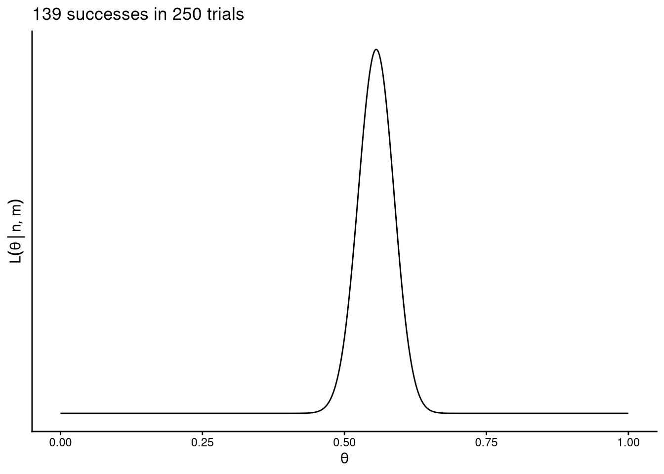

m <- 14
n <- 25
bernoulli_likelihood(n, m)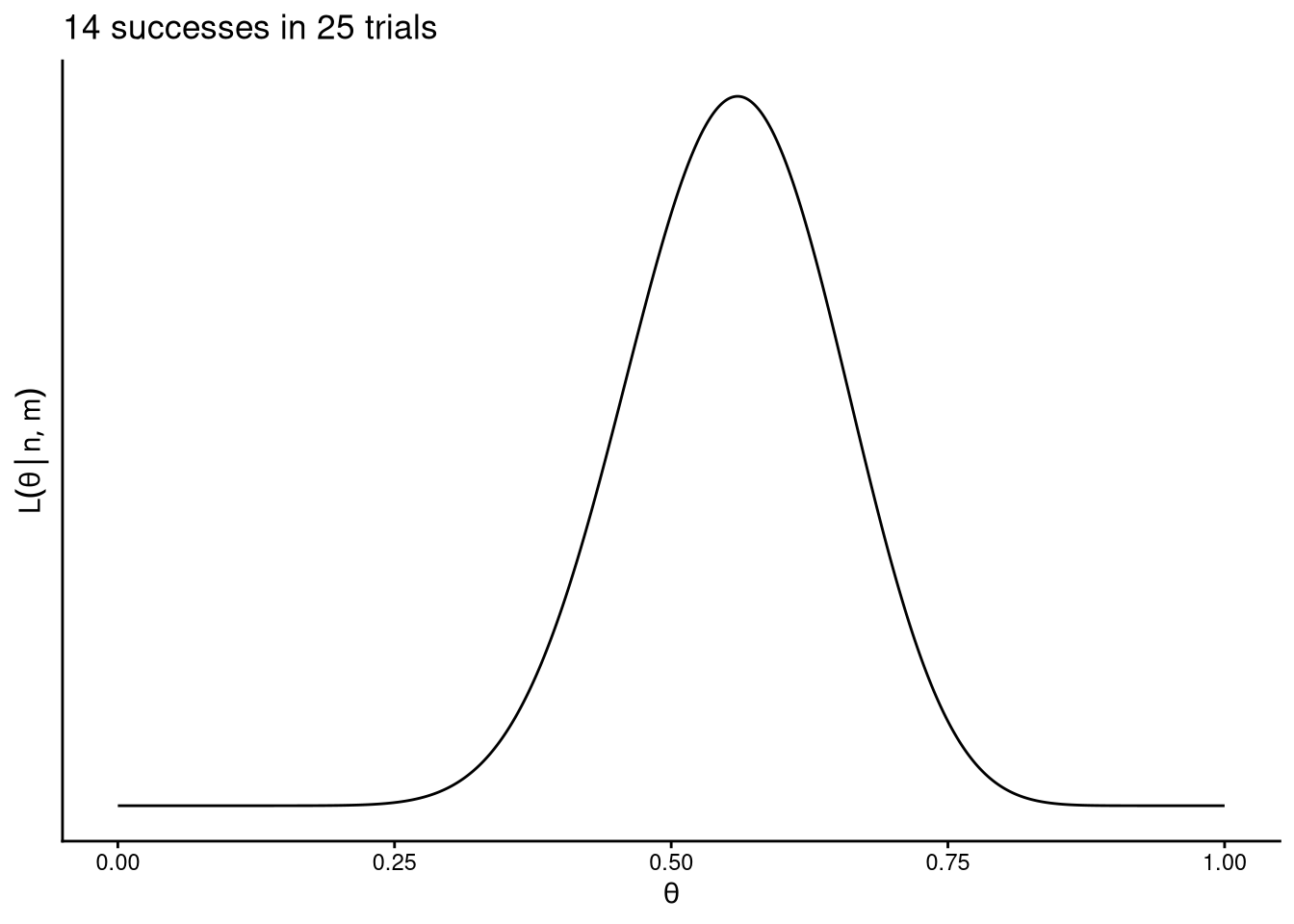

The two examples above show the same proportion of successes (\(m/n \approx 0.56\)) but different sample sizes. The second curve is wider, reflecting greater uncertainty when fewer observations are available.

The beta distribution as prior

We need a prior distribution on \(\theta\), a probability distribution over the interval \([0, 1]\). The beta distribution is a natural choice. It has two shape parameters, \(\alpha\) and \(\beta\), and its density is

\[ p(\theta) \propto \theta^{\alpha - 1} (1 - \theta)^{\beta - 1} \]

Different values of \(\alpha\) and \(\beta\) produce very different shapes.

beta_plot(alpha = 1, beta = 1) # uniform: no prior information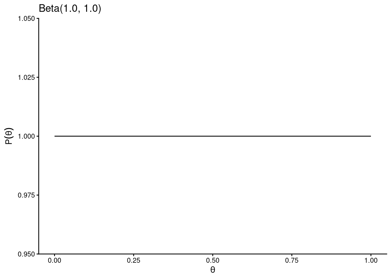

beta_plot(alpha = 3, beta = 5) # mild preference for values below 0.5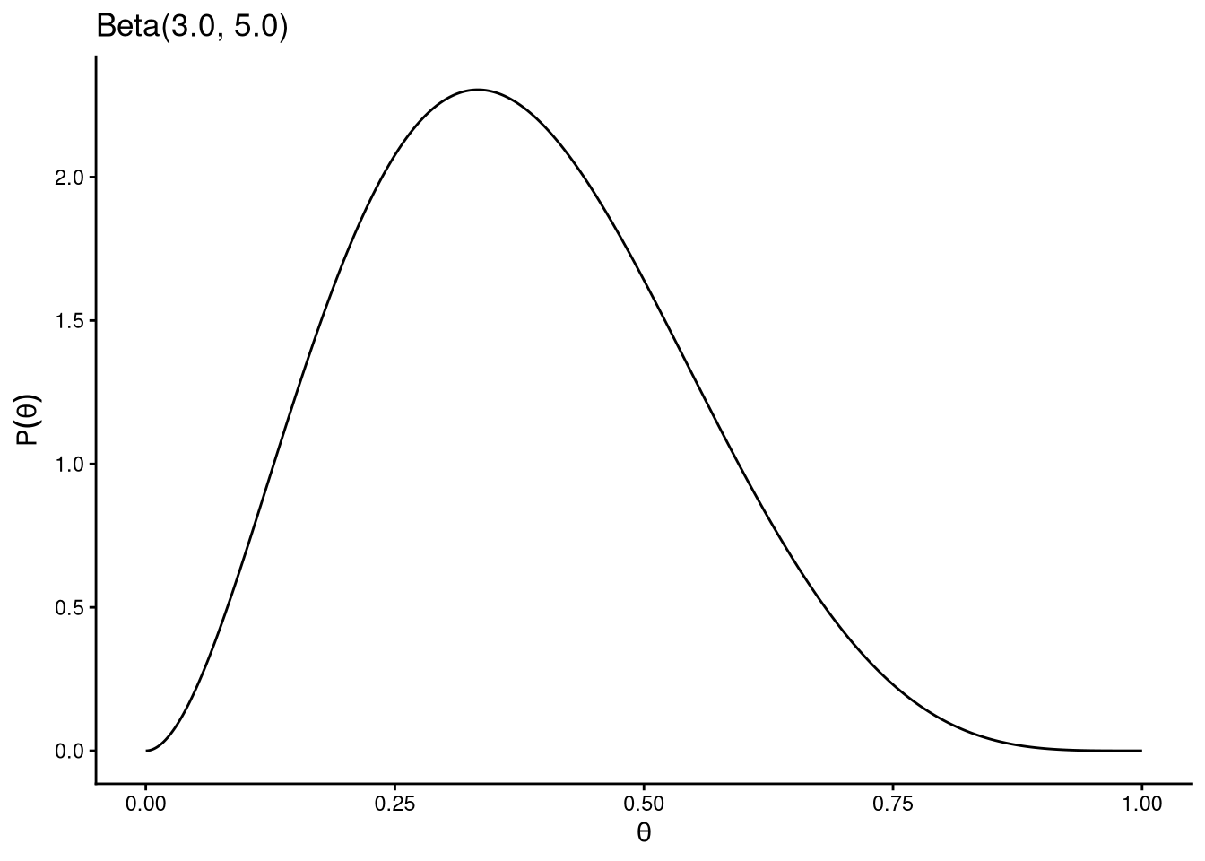

beta_plot(alpha = 5, beta = 3) # mild preference for values above 0.5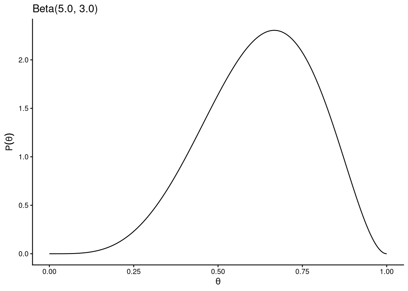

beta_plot(alpha = 9, beta = 15) # stronger preference for values around 0.37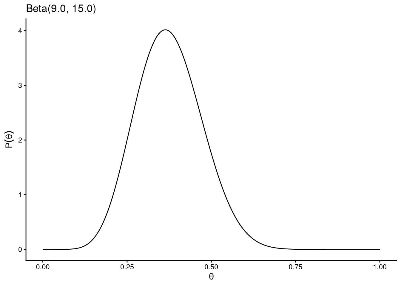

The uniform prior \(\text{Beta}(1, 1)\) represents complete ignorance: all values of \(\theta\) are equally plausible before seeing the data. Other choices encode prior knowledge: if we know from previous studies that the probability is likely below 0.5, a prior like \(\text{Beta}(3, 5)\) captures that belief.

Conjugacy

The beta distribution has a convenient property called conjugacy with respect to the binomial likelihood. When the prior is \(\text{Beta}(\alpha, \beta)\) and we observe \(m\) successes in \(n\) trials, the posterior is

\[ \theta \mid m, n \sim \text{Beta}(\alpha + m,\; \beta + n - m) \]

The posterior parameters are the prior parameters plus the observed counts. This means we can compute the posterior analytically, without numerical integration. The prior parameters \(\alpha\) and \(\beta\) act like pseudo-counts: \(\alpha\) is the prior equivalent of seeing \(\alpha - 1\) additional successes and \(\beta - 1\) additional failures.

This conjugacy is pedagogically valuable because it lets us see exactly how the prior and the likelihood combine to form the posterior. In the next session we will work through this in detail.